This is documentation for the next version of Grafana documentation. For the latest stable release, go to the latest version.

Documentation Grafana documentation Data sources Microsoft SQL Server Query editor

Microsoft SQL Server query editor

Grafana provides a query editor for the Microsoft SQL Server data source, which is located on the Explore page. You can also access the MSSQL query editor from a dashboard panel. Click the menu in the upper right of the panel and select Edit.

This topic explains querying specific to the MSSQL data source. For general documentation on querying data sources in Grafana, refer to Query and transform data. For options and functions common to all query editors, refer to Query editors.

For more information on writing Transact-SQL statements, refer to Write Transact-SQL statements and Transact-SQL reference in the Microsoft SQL Server documentation.

The Microsoft SQL Server query editor has two modes:

• Builder mode
• Code mode

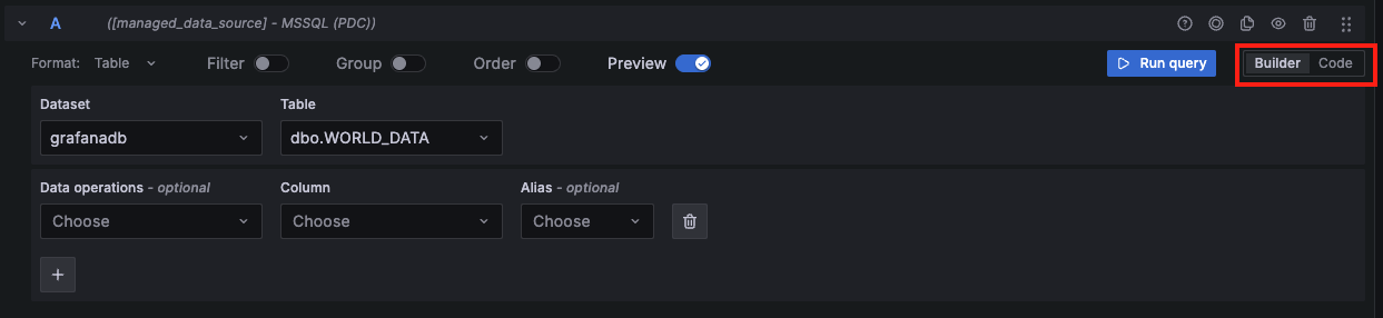
To switch between the editor modes, select the corresponding Builder and Code tabs in the upper right.

To run a query, select Run query in the upper right of the editor.

In addition to writing queries, the query editor also allows you to create and use:

• Macros
• Annotations
• Stored procedures

Builder mode

Builder mode allows you to build queries using a visual interface. This mode is great for users who prefer a guided query experience or are just getting started with SQL.

The following components will help you build a T-SQL query:

• Format - Select a format response from the drop-down for the MSSQL query. The default is Table. Refer to Table queries and Time series queries for more information and examples. If you select the Time series format option, you must include a time column.

• Dataset - Select a database to query from the drop-down. Grafana automatically populates the drop-down with all databases the user has access to. If a default database is configured in the Data Source Configuration page or via a provisioning file, users will be limited to querying only that predefined database.

  Note that tempdb, model, msdb, and master system databases are not included in the query editor drop-down.

• Table - Select a table from the drop-down. After selecting a database, the next drop-down displays all available tables in that database.

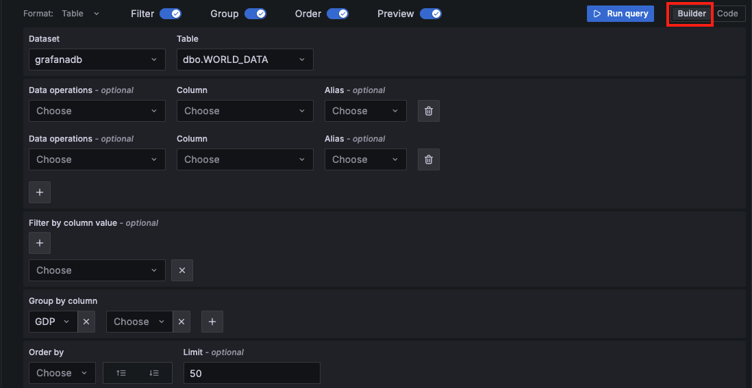
• Data operations - Optional. Select an aggregation or a macro from the drop-down. You can add multiple data operations by clicking the + sign. Click the garbage can icon to remove data operations.

  • Column - Select a column on which to run the aggregation.
  • Interval - Select an interval from the drop-down. You’ll see this option when you choose a time group macro from the drop-down.
  • Fill - Optional. Add a FILL method to populate missing time intervals with default values (such as NULL, 0, or a specified value) when no data exists for those intervals. This ensures continuity in the time series, avoiding gaps in visualizations.
  • Alias - Optional. Add an alias from the drop-down. You can also add your own alias by typing it in the box and clicking Enter. Remove an alias by clicking the X.

• Filter - Toggle to add filters.

  • Filter by column value - Optional. If you toggle Filter you can add a column to filter by from the drop-down. To filter by additional columns, click the + sign to the right of the condition drop-down. You can choose a variety of operators from the drop-down next to the condition. When multiple filters are added, use the AND or OR operators to define how conditions are evaluated. AND requires all conditions to be true, while OR requires any condition to be true. Use the second drop-down to select the filter value. To remove a filter, click the X icon next to it. If you select a date-type column, you can use macros from the operator list and choose timeFilter to insert the $\_\_timeFilter macro into your query with the selected date column.

    After selecting a date type column, you can choose Macros from the operators list and select timeFilter which will add the $\_\_timeFilter macro to the query with the selected date column. Refer to Macros for more information.

• Group - Toggle to add a GROUP BY column.

  • Group by column - Select a column to filter by from the drop-down. Click the +sign to filter by multiple columns. Click the X to remove a filter.

• Order - Toggle to add an ORDER BY statement.

  • Order by - Select a column to order by from the drop-down. Select ascending (ASC) or descending (DESC) order.
  • Limit - You can add an optional limit on the number of retrieved results. Default is 50.

• Preview - Toggle for a preview of the SQL query generated by the query builder. Preview is toggled on by default.

For additional detail about using formats, refer to Table queries and Time series queries.

Code mode

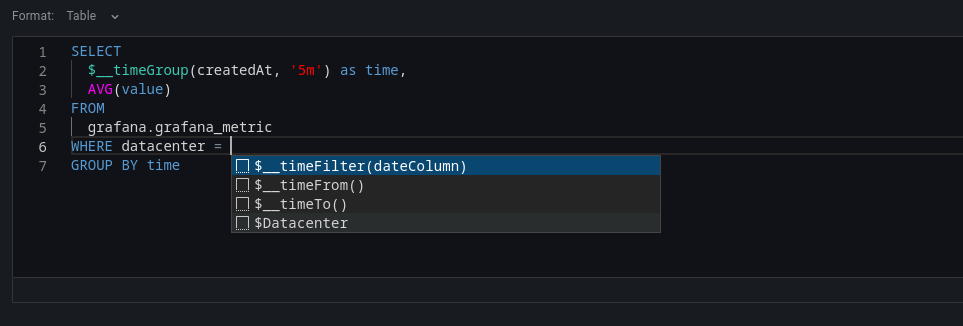
Code mode lets you build complex queries using a text editor with helpful features like autocompletion and syntax highlighting.

This mode is ideal for advanced users who need full control over the SQL query or want to use features not available in visual query mode. It’s especially useful for writing subqueries, using macros, or applying advanced filtering and formatting. You can switch back to visual mode, but note that some custom queries may not be fully compatible.

Code mode toolbar features

Code mode has several features in a toolbar located in the editor’s lower-right corner.

• To reformat the query, click the brackets button ({}).
• To expand the code editor, click the chevron button pointing downward.
• To run the query, click the Run query button or use the keyboard shortcut Ctrl/Cmd + Enter/Return.

Use autocompletion

Code mode’s autocompletion feature works automatically while typing. To manually trigger autocompletion, use the keyboard shortcut Ctrl/Cmd + Space.

Code mode supports autocompletion of tables, columns, SQL keywords, standard SQL functions, Grafana template variables, and Grafana macros.

Macros

To simplify syntax and to allow for dynamic components, such as date range filters, you can add macros to your query.

Use macros in the SELECT clause to simplify the creation of time series queries. From the Data operations drop-down, choose a macro such as $\_\_timeGroup or $\_\_timeGroupAlias. Then, select a time column from the Column drop-down and a time interval from the Interval drop-down. This generates a time-series query based on your selected time grouping.

View the interpolated query

The query editor includes a Generated SQL link that appears after you run a query while editing a panel. Click this link to view the raw interpolated SQL that Grafana executed, including any macros that were expanded during query processing.

Table queries

To create a Table query, set the Format option in the query editor to Table. This allows you to write any valid SQL query, and the Table panel will display the results using the returned columns and rows.

Example:

sql Copy

CREATE TABLE [event] (
  time_sec bigint,
  description nvarchar(100),
  tags nvarchar(100),
)

sql Copy

CREATE TABLE [mssql_types] (
  c_bit bit, c_tinyint tinyint, c_smallint smallint, c_int int, c_bigint bigint, c_money money, c_smallmoney smallmoney, c_numeric numeric(10,5),
  c_real real, c_decimal decimal(10,2), c_float float,
  c_char char(10), c_varchar varchar(10), c_text text,
  c_nchar nchar(12), c_nvarchar nvarchar(12), c_ntext ntext,
  c_datetime datetime,  c_datetime2 datetime2, c_smalldatetime smalldatetime, c_date date, c_time time, c_datetimeoffset datetimeoffset
)

INSERT INTO [mssql_types]
SELECT
  1, 5, 20020, 980300, 1420070400, '$20000.15', '£2.15', 12345.12,
  1.11, 2.22, 3.33,
  'char10', 'varchar10', 'text',
  N'☺nchar12☺', N'☺nvarchar12☺', N'☺text☺',
  GETDATE(), CAST(GETDATE() AS DATETIME2), CAST(GETDATE() AS SMALLDATETIME), CAST(GETDATE() AS DATE), CAST(GETDATE() AS TIME), SWITCHOFFSET(CAST(GETDATE() AS DATETIMEOFFSET), '-07:00')

Example query with output:

sql Copy

SELECT * FROM [mssql_types]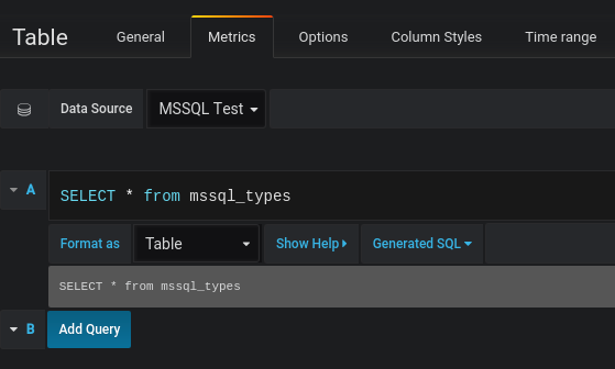

Use the keyword AS to define an alias in your query to rename a column or table.

Example query with output:

sql Copy

SELECT
  c_bit AS [column1], c_tinyint AS [column2]
FROM
  [mssql_types]

Time series queries

To create a time series query, set the Format option in the query editor to Time series. The query must include a column named time, which should contain either a SQL datetime value or a numeric value representing Unix epoch time in seconds. The result set must be sorted by the time column for panels to visualize the data correctly.

A time series query returns resultswide data frame format.

• Any column except time or of the type string transforms into value fields in the data frame query result.
• Any string column transforms into field labels in the data frame query result.

You can enable macro support in the SELECT clause to create time series queries more easily. Use the Data operations drop-down to choose a macro such as $\_\_timeGroup or $\_\_timeGroupAlias, then select a time column from the Column drop-down and a time interval from the Interval drop-down. This generates a time-series query based on your selected time grouping.

Macros

You can enable macros support in the select clause to create time-series queries.

Use the Data operations drop-down to select a macro like $__timeGroup or $__timeGroupAlias. Select a time column from the Column drop-down and a time interval from the Interval drop-down to create a time-series query.

You can also add custom value to the Data operations. For example, a function that’s not in the drop-down list. This allows you to add any number of parameters.

Create a metric query

For backward compatibility, there’s an exception to the above rule for queries that return three columns and include a string column named metric. Instead of transforming the metric column into field labels, it becomes the field name, and then the series name is formatted as the value of the metric column. See the example with the metric column below.

To optionally customize the default series name formatting, refer to Standard options definitions.

Example with metric column:

sql Copy

SELECT
  $__timeGroupAlias(time_date_time, '5m'),
  min("value_double"),
  'min' as metric
FROM test_data
WHERE $__timeFilter(time_date_time)
GROUP BY time
ORDER BY 1

Data frame result:

text Copy

+---------------------+-----------------+
| Name: time          | Name: min       |
| Labels:             | Labels:         |
| Type: []time.Time   | Type: []float64 |
+---------------------+-----------------+
| 2020-01-02 03:05:00 | 3               |
| 2020-01-02 03:10:00 | 6               |
+---------------------+-----------------+

Time series query examples

Use the fill parameter in the $__timeGroupAlias macro to convert null values to be zero instead:

sql Copy

SELECT
  $__timeGroupAlias(createdAt, '5m', 0),
  sum(value) as value,
  hostname
FROM test_data
WHERE
  $__timeFilter(createdAt)
GROUP BY
  time,
  hostname
ORDER BY 1

Given the data frame result in the following example and using the graph panel, you will get two series named value 10.0.1.1 and value 10.0.1.2. To render the series with a name of 10.0.1.1 and 10.0.1.2 , use a Standard options definitions display name value of ${__field.labels.hostname}.

Data frame result:

text Copy

+---------------------+---------------------------+---------------------------+
| Name: time          | Name: value               | Name: value               |
| Labels:             | Labels: hostname=10.0.1.1 | Labels: hostname=10.0.1.2 |
| Type: []time.Time   | Type: []float64           | Type: []float64           |
+---------------------+---------------------------+---------------------------+
| 2020-01-02 03:05:00 | 3                         | 4                         |
| 2020-01-02 03:10:00 | 6                         | 7                         |
+---------------------+---------------------------+---------------------------+

Use multiple columns:

sql Copy

SELECT
  $__timeGroupAlias(time_date_time, '5m'),
  min(value_double) as min_value,
  max(value_double) as max_value
FROM test_data
WHERE $__timeFilter(time_date_time)
GROUP BY time
ORDER BY 1

Data frame result:

text Copy

+---------------------+-----------------+-----------------+
| Name: time          | Name: min_value | Name: max_value |
| Labels:             | Labels:         | Labels:         |
| Type: []time.Time   | Type: []float64 | Type: []float64 |
+---------------------+-----------------+-----------------+
| 2020-01-02 03:04:00 | 3               | 4               |
| 2020-01-02 03:05:00 | 6               | 7               |
+---------------------+-----------------+-----------------+

Apply annotations

Annotations overlay rich event information on top of graphs. You can add annotation queries in the Dashboard menu’s Annotations view.

Columns:

Example database tables:

sql Copy

CREATE TABLE [events] (
  time_sec bigint,
  description nvarchar(100),
  tags nvarchar(100),
)

The following example also uses the database table defined in the Time series queries section.

Example query using time column with epoch values:

sql Copy

SELECT
  time_sec as time,
  description as [text],
  tags
FROM
  [events]
WHERE
  $__unixEpochFilter(time_sec)
ORDER BY 1

Example region query using time and timeend columns with epoch values:

sql Copy

SELECT
  time_sec as time,
  time_end_sec as timeend,
  description as [text],
  tags
FROM
  [events]
WHERE
  $__unixEpochFilter(time_sec)
ORDER BY 1

Example query using time column of native SQL date/time data type:

sql Copy

SELECT
  time,
  measurement as text,
  convert(varchar, valueOne) + ',' + convert(varchar, valueTwo) as tags
FROM
  metric_values
WHERE
  $__timeFilter(time_column)
ORDER BY 1

Use stored procedures

Stored procedures have been verified to work with Grafana queries. However, note that there is no special handling or extended support for stored procedures, so some edge cases may not behave as expected.

Stored procedures can be used in table, time series, and annotation queries, provided that the returned data matches the expected column names and formats described in the relevant previous sections in this document.

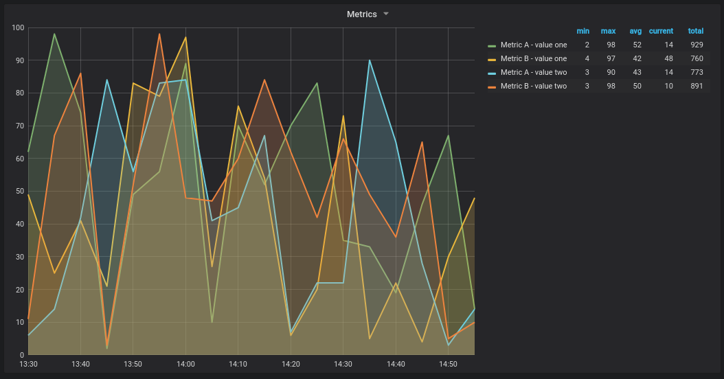
For the following examples, the database table is defined in Time series queries. Let’s say that we want to visualize four series in a graph panel, such as all combinations of columns valueOne, valueTwo and measurement. Graph panel to the right visualizes what we want to achieve. To solve this, you need to use two queries:

First query:

sql Copy

SELECT
  $__timeGroup(time, '5m') as time,
  measurement + ' - value one' as metric,
  avg(valueOne) as valueOne
FROM
  metric_values
WHERE
  $__timeFilter(time)
GROUP BY
  $__timeGroup(time, '5m'),
  measurement
ORDER BY 1

Second query:

sql Copy

SELECT
  $__timeGroup(time, '5m') as time,
  measurement + ' - value two' as metric,
  avg(valueTwo) as valueTwo
FROM
  metric_values
GROUP BY
  $__timeGroup(time, '5m'),
  measurement
ORDER BY 1

Stored procedure with epoch time format

You can define a stored procedure to return all the data needed to render multiple series (for example, 4) in a graph panel.

In the following example, the stored procedure accepts two parameters, @from and @to, both of type int. These parameters represent a time range (from–to) in epoch time format and are used to filter the results returned by the procedure.

The query inside the procedure simulates the behavior of $__timeGroup(time, '5m') by grouping timestamps into 5-minute intervals. While the expressions for time grouping are somewhat verbose, they can be extracted into reusable SQL Server functions to simplify the procedure.

sql Copy

CREATE PROCEDURE sp_test_epoch(
  @from int,
  @to 	int
)	AS
BEGIN
  SELECT
    cast(cast(DATEDIFF(second, {d '1970-01-01'}, DATEADD(second, DATEDIFF(second,GETDATE(),GETUTCDATE()), time))/600 as int)*600 as int) as time,
    measurement + ' - value one' as metric,
    avg(valueOne) as value
  FROM
    metric_values
  WHERE
    time >= DATEADD(s, @from, '1970-01-01') AND time <= DATEADD(s, @to, '1970-01-01')
  GROUP BY
    cast(cast(DATEDIFF(second, {d '1970-01-01'}, DATEADD(second, DATEDIFF(second,GETDATE(),GETUTCDATE()), time))/600 as int)*600 as int),
    measurement
  UNION ALL
  SELECT
    cast(cast(DATEDIFF(second, {d '1970-01-01'}, DATEADD(second, DATEDIFF(second,GETDATE(),GETUTCDATE()), time))/600 as int)*600 as int) as time,
    measurement + ' - value two' as metric,
    avg(valueTwo) as value
  FROM
    metric_values
  WHERE
    time >= DATEADD(s, @from, '1970-01-01') AND time <= DATEADD(s, @to, '1970-01-01')
  GROUP BY
    cast(cast(DATEDIFF(second, {d '1970-01-01'}, DATEADD(second, DATEDIFF(second,GETDATE(),GETUTCDATE()), time))/600 as int)*600 as int),
    measurement
  ORDER BY 1
END

Then, in your graph panel, you can use the following query to call the stored procedure with the time range dynamically populated by Grafana:

sql Copy

DECLARE
  @from int = $__unixEpochFrom(),
  @to int = $__unixEpochTo()

EXEC dbo.sp_test_epoch @from, @to

This uses Grafana built-in macros to convert the selected time range into epoch time ($**unixEpochFrom() and $**unixEpochTo()), which are passed to the stored procedure as input parameters.

Stored procedure with datetime format

You can define a stored procedure to return all the data needed to render four series in a graph panel.

In the following example, the stored procedure accepts two parameters, @from and @to, of the type datetime. These parameters represent the selected time range and are used to filter the returned data.

The query within the procedure mimics the behavior of $__timeGroup(time, '5m') by grouping data into 5-minute intervals. These expressions can be verbose, but you may extract them into reusable SQL Server functions for improved readability and maintainability.

sql Copy

CREATE PROCEDURE sp_test_datetime(
  @from datetime,
  @to 	datetime
)	AS
BEGIN
  SELECT
    cast(cast(DATEDIFF(second, {d '1970-01-01'}, time)/600 as int)*600 as int) as time,
    measurement + ' - value one' as metric,
    avg(valueOne) as value
  FROM
    metric_values
  WHERE
    time >= @from AND time <= @to
  GROUP BY
    cast(cast(DATEDIFF(second, {d '1970-01-01'}, time)/600 as int)*600 as int),
    measurement
  UNION ALL
  SELECT
    cast(cast(DATEDIFF(second, {d '1970-01-01'}, time)/600 as int)*600 as int) as time,
    measurement + ' - value two' as metric,
    avg(valueTwo) as value
  FROM
    metric_values
  WHERE
    time >= @from AND time <= @to
  GROUP BY
    cast(cast(DATEDIFF(second, {d '1970-01-01'}, time)/600 as int)*600 as int),
    measurement
  ORDER BY 1
END

To call this stored procedure from a graph panel, use the following query with Grafana built-in macros to populate the time range dynamically:

sql Copy

DECLARE
  @from datetime = $__timeFrom(),
  @to datetime = $__timeTo()

EXEC dbo.sp_test_datetime @from, @to