How to create Grafana alerts with InfluxDB and the Flux query language
By Grant Pinkos
Last update on July 18, 2023
Introduction
Grafana Alerting represents a powerful new approach to systems observability and incident response management. While the alerting platform is perhaps best known for its strong integrations with Prometheus, the system works with numerous popular data sources including InfluxDB. In this tutorial we will learn how to create Grafana alerts using InfluxDB and the newer Flux query language. We will cover five common scenarios from the most basic to the most complex. Together, these five scenarios will provide an excellent guide for almost any type of alerting query that you wish to create using Grafana and Flux.
Before we dive into our alerting scenarios, it is worth considering the development of InfluxDB’s two popular query languages: InfluxQL and Flux. Originally, InfluxDB used InfluxQL as their query language, which uses a SQL-like syntax. But beginning with InfluxDB v1.8, the company introduced Flux, “an open source functional data scripting language designed for querying, analyzing, and acting on data.” “Flux,” its official documentation goes on to state, “unifies code for querying, processing, writing, and acting on data into a single syntax. The language is designed to be usable, readable, flexible, composable, testable, contributable, and shareable.”
In the following five examples we will see just how powerful and flexible the new Flux query language can be. We will also see just how well Flux pairs with Grafana Alerting.
Example 1: Create an alert when a value is above or below a set threshold
Our first example uses a common real-world scenario for InfluxDB and Grafana Alerting. Popular with IoT and edge applications, InfluxDB excels at on-site, real-time observability. In this example, and in fact for many of the following examples, we will consider the hypothetical scenario where we are monitoring a number of fluid tanks in a manufacturing plant. This scenario, based on an actual application of InfluxDB and Alerting, will allow us to work through Grafana’s various alerting setups, progressing from the simplest to the most complex.
For Example 1, let’s consider the following scenario: we are monitoring one tank, A5, for which we are storing real-time temperature data. We need to make sure that the temperature in this tank is always greater than 30 °C and less than 60 °C.
We want to write a Grafana alert that will trigger whenever the temperature in tank A5 crosses the lower threshold of 30 °C or the upper threshold of 60 °C.
To do this, we’ll: create a Grafana alert rule, add a Flux query, and then add expressions to the alert rule.
Create a Grafana Alert rule
- Open the Grafana alerting menu and select Alert rules.
- Click New alert rule.
- Give your alert rule a name and then select Grafana managed alert. For InfluxDB, you will always create a Grafana managed rule.
Add an initial Flux query to the alert rule
Still in the Step 2 section of the Alert rule page, you will see three boxes: a query editor (A), and then two sections labelled B and C. You will use these three sections to construct your rule. Let’s move through them one by one.
First, we want to query the data in our imaginary InfluxDB instance to obtain a time series graph of the temperature of tank A5. For this you would choose your InfluxDB data source from the dropdown and then write a query like this:
```
 from(bucket: "RetroEncabulator")
|> range(start: v.timeRangeStart, stop: v.timeRangeStop)
|> filter(fn: (r) => r["_measurement"] == "TemperatureData")
|> filter(fn: (r) => r["Tank"] == "A5")
|> filter(fn: (r) => r["_field"] == "Temperature")
|> aggregateWindow(every: v.windowPeriod, fn: mean, createEmpty: false)
|> yield(name: "mean")
```
This is a fairly typical Flux query. Let’s go through it function by function. We begin using the from() function to choose the correct bucket where our tank data resides. Then we use a range() function to filter our rows based on time constraints. Then we pass our data through three filter() functions to narrow our results. We choose a specific measurement (a special keyword in InfluxDB), then our tank in question (A5), and then a specific field (another special keyword in InfluxDB). After this we pass the data into an aggregateWindow() function, which downsamples our data into specific periods of time, and then finally a yield() function, which specifies which final result we want: mean.
This Flux query will yield a time-series graph like this:
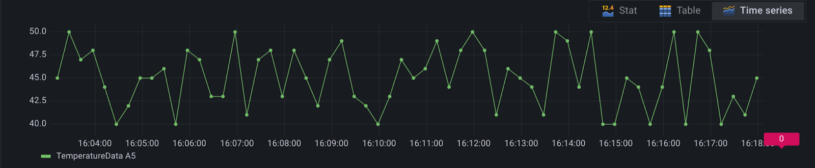
Add expressions to your Grafana Alert rule
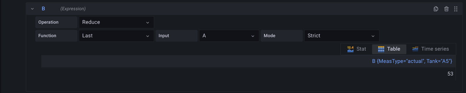
With data now appearing in our rule setup, our next step is to create an expression. Move to section B. For this scenario, we want to create a Reduce expression that will reduce the above to a single value. In this image, you can see that we have chosen to reduce our time-series data the Last value from input A. In this case, it returns a value 53 degrees celsius for Tank A5:
Finally, we need to create a math expression that Grafana will alert on. In our case we will write an expression with two conditions separated by the OR || operator. We want to trigger an alert any time our result in section B is less than 30 or more than 60. This looks like $B < 30 || $B > 60:
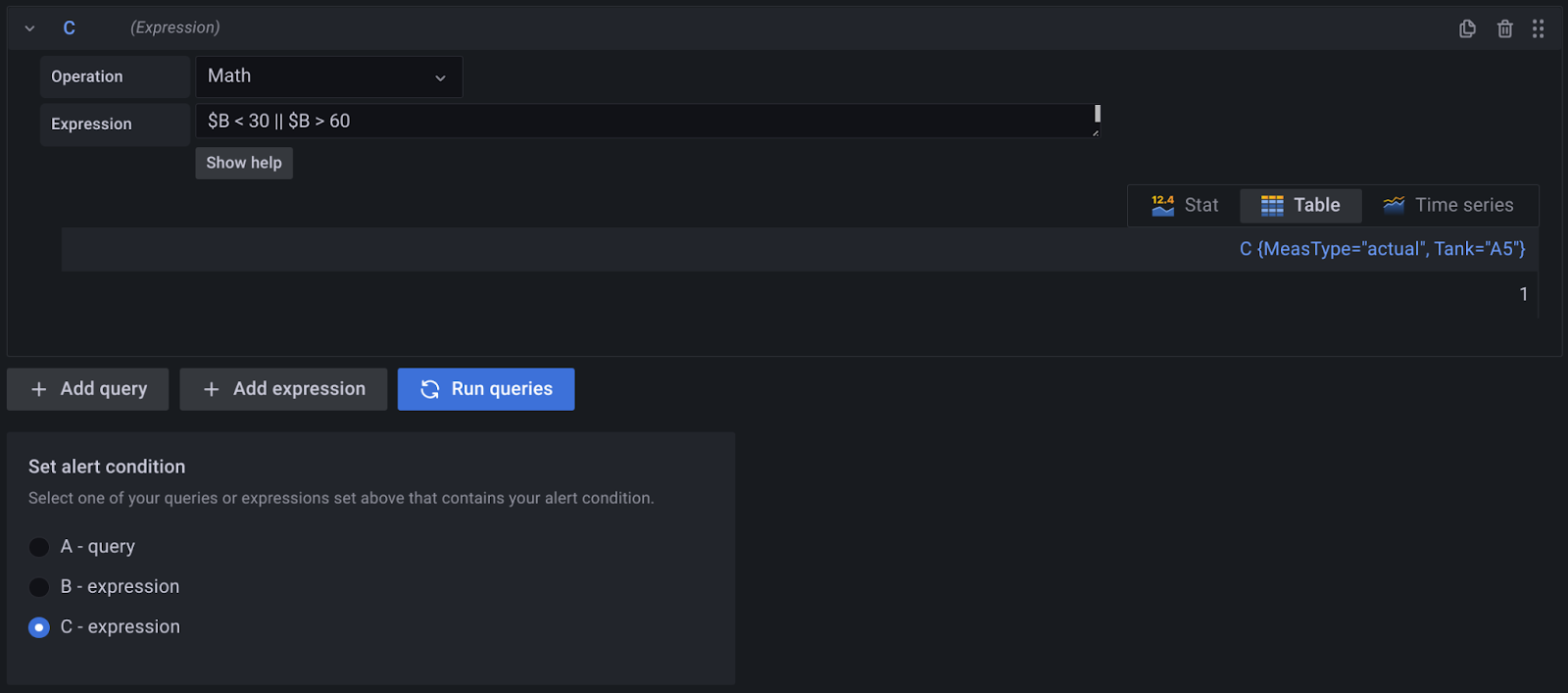
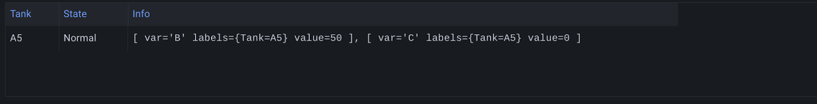
Set the alert condition to C - expression. We can now preview our alert. Here is a preview of this alert when the state is Normal:
And here is a preview of this alert when the state is Alerting:
Note that the Reduce expression above is needed. Without it, when previewing the results, Grafana would display invalid format of evaluation results for the alert definition B: looks like time series data, only reduced data can be alerted on.
💡Tip: In case your locale is still stubbornly using Fahrenheit, we can modify the above Flux query by adding (before the aggregateWindow statement) a map() function to to convert (or map) the values from °C to °F. Note that we are not creating a new field. We are simply remapping the existing value.
|> map(fn: (r) => ({r with _value: r._value * 1.8 + 32.0}))Conclusion
Using these three steps you can create a Flux-based Grafana Alert that will trigger on either of two thresholds from a single data source. But what if you need to trigger an alert based on multiple conditions and from multiple time-series? In example two we will cover this very scenario.
Example 2: how to create a Grafana alert from two queries and two conditions
Let’s mix things up a bit for example two and leave our imaginary manufacturing plant. Imagine you’re an assistant to the great Dr. Emmett Brown from Back to the Future, and Doc has tasked you with the following challenge: “I want an alert sent to me every time both conditions for time travel are met: when the velocity of a vehicle reaches 88 miles per hour and an object generates 1.21 jigowatts of electricity.”
Let’s assume we are tracking this data in InfluxDB and Grafana. Let’s also assume that each of the above data sources comes from different buckets. How do we alert on this? How do we use Grafana and Flux to alert on two distinct conditions originating from two distinct data sources?
Add two Flux queries to your Grafana Alert rule
Like we did in example 1, let’s first mock up our queries. Our query for our vehicle data is very similar to our last query. We use a from(), range(), and a sequence of filter() functions. We then use AggregateWindow() and yield() to narrow our data even more. In this case, the result is a time series tracking the velocity of our 1983 DeLorean:
from(bucket: "vehicles")
|> range(start: v.timeRangeStart, stop: v.timeRangeStop)
|> filter(fn: (r) => r["_measurement"] == "VehicleData")
|> filter(fn: (r) => r["VehicleType"] == "DeLorean")
|> filter(fn: (r) => r["VehicleYear"] == "1983")
|> filter(fn: (r) => r["_field"] == "velocity")
|> aggregateWindow(every: v.windowPeriod, fn: mean, createEmpty: false)
|> yield(name: "mean")
Our second query will trigger an alert whenever our electricity resource (the lightning strike on the Hill Valley clocktower) reaches the needed 1.21 jigowatts. A query like this would look very similar to our vehicle velocity query:
from(bucket: "HillValley")
|> range(start: v.timeRangeStart, stop: v.timeRangeStop)
|> filter(fn: (r) => r["_measurement"] == "ElectricityData")
|> filter(fn: (r) => r["Location"] == "clocktower")
|> filter(fn: (r) => r["Source"] == "lightning")
|> filter(fn: (r) => r["_field"] == "power")
|> aggregateWindow(every: v.windowPeriod, fn: mean, createEmpty: false)
|> yield(name: "mean")
We are now ready to modify this data using expressions.
Add expressions to your Grafana Alert rule
Let’s now use the same steps to reduce each query to the last (most recent) value. Reducing Query
Ato a single value might look like this:![grafana alerts from flux queries]()
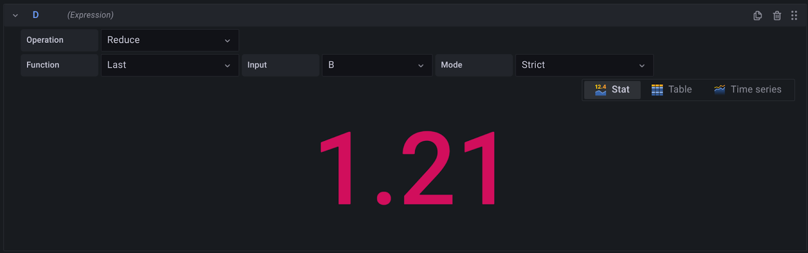
And here we are reducing query
B:![grafana alerts from flux queries]()
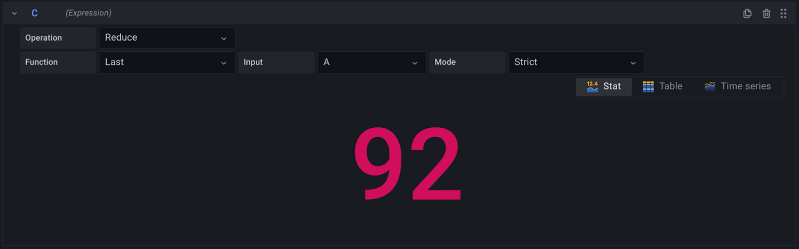
Now, in section
Cwe need to create a math expression to be alerted on. In this case we will use the AND&&operator to specify that two conditions must be met: the value ofC(the reduced value from queryA) must be greater than 88.0 while the value ofD(the reduced value from queryB) must be greater than 1.21. We write this as$C > 88.0 && $D > 1.21![grafana alerts from flux queries]()

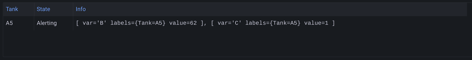
And here is a preview of our alerts:

💡Tip: If your data in InfluxDB happens to have an unnecessarily large number of digits to the right of the decimal (such as 1.2104705741732575 shown above), and you want your Grafana alerts to be more legible, try using {{ printf “%.2f” $values.D.Value }}. For example, in the annotation Summary, we could write the following:
{{ $values.D.Labels.Source }} at the {{ $values.D.Labels.Location }} has generated {{ printf "%.2f" $values.D.Value }} jigowatts.`This will display as follows:
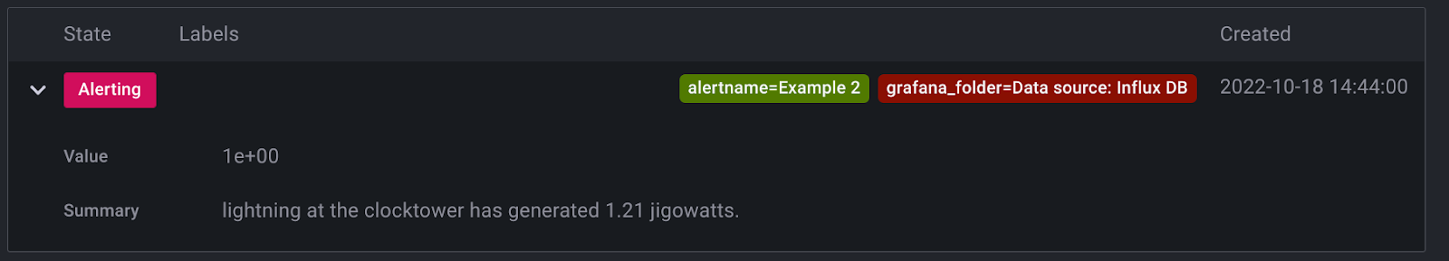 )
)
You can reference our documentation on alert message templating to learn more about this powerful feature.
Conclusion
In this example we showed how to create a Flux-based alert that uses two distinct conditions from two distinct queries that use data from two distinct data sources. For example three we will switch gears and tackle another popular alerting scenario: how to create an alert based on an aggregated (per day) value.
Example 3: how to create a Grafana Alert based on an aggregated (per-day) value
One of the most common requests in Grafana’s community forum involves graphing daily electrical consumption and production. This sort of data is very often stored in InfluxDB. In this example we will see how to aggregate time series data into a per-day value and then alert on it.
Let’s assume our electricity meter sends a reading to InfluxDB once per hour and contains the total kWh used for that hour. We want to write a query that will aggregate these per-hour values into a per-day value, then create an alert that triggers when the power consumption (kWh) exceeds 5,000 kWh per day.
Add an initial Flux query to your Grafana Alert rule
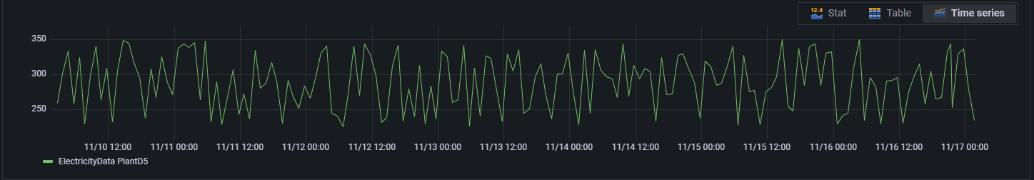
Let’s begin by examining a typical query and the resulting time graph for our hourly data across a 7-day period. A query like this is shown below:
from(bucket: "RetroEncabulator")
|> range(start: v.timeRangeStart, stop: v.timeRangeStop)
|> filter(fn: (r) => r["_measurement"] == "ElectricityData")
|> filter(fn: (r) => r["Location"] == "PlantD5")
|> filter(fn: (r) => r["_field"] == "power_consumed")
|> aggregateWindow(every: v.windowPeriod, fn: mean, createEmpty: false)
|> yield(name: "power")
We can see the same pattern of Flux functions here that we say in examples 1 and 2. A query like this would produce a graph similar to the following:
![grafana alerts from flux queries]()
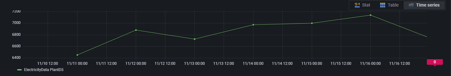
Now let’s adjust our query to calculate daily usage. With many datasources, this can be a rather complex operation. But with Flux, by simply changing the aggregateWindow function parameters we can calculate the daily usage over the same 7-day period:
from(bucket: "RetroEncabulator")
  |> range(start: v.timeRangeStart, stop: v.timeRangeStop)
  |> filter(fn: (r) => r["_measurement"] == "ElectricityData")
  |> filter(fn: (r) => r["Location"] == "PlantD5")
  |> filter(fn: (r) => r["_field"] == "power_consumed")
  |> aggregateWindow(every: 1d, fn: sum)
  |> yield(name: "power")
Note how we’ve adjusted our
aggregateWindow()function toaggregateWindow(every: 1d, fn: sum). This results in a graph like so:![grafana alerts from flux queries]()
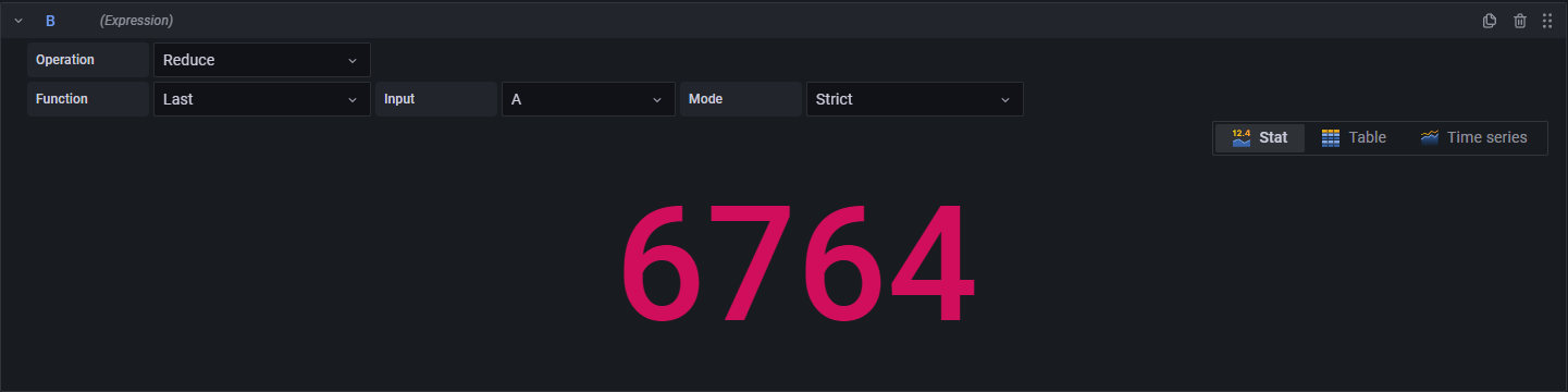
Add expressions to your Grafana Alert rule.
Now that we have our per-day query correct, we can continue using the same pattern as before, adding expressions to reduce and perform math on our results.
As before, let’s reduce our query to a single value:
![grafana alerts from flux queries]()
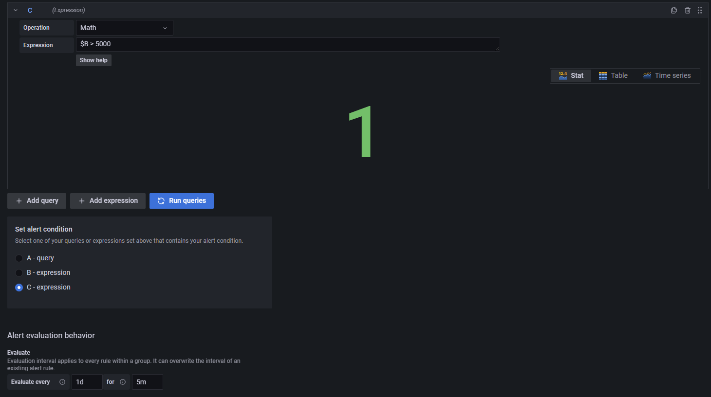
Now create a math expression to be alerted on and set the evaluation behavior. In this case we want to write
$B > 5000:![grafana alerts from flux queries]()
And now we are alerting on our daily electricity consumption whenever we exceed 5000 kWh. Here is preview of our alert:
![grafana alerts from flux queries]()

Conclusion
Plotting and aggregating electrical consumption is a common use case for combining InfluxDB and Grafana. Using Flux, we saw just how easy it can be to group our data by day and then alert on that daily value. In our next two examples we will examine the more complex form of Grafana Alert: multidimensional alerts.
Example 4: create a dynamic (multidimensional) Grafana Alert using Flux
Let’s return to our fluid tanks from example 1, but this time let’s assume we have 5 tanks (A5, B4, C3, D2, and E1). We are now tracking the temperature in five tanks: A5, B4, C3, D2, and E1.
We want to create one multidimensional alert that will notify us whenever the temperature in any tank is less than 30 °C or greater than 60 °C.
Add an initial Flux query to your Grafana Alert rule
We begin, as always, by writing our initial query. This is very similar to our query in example 1, but note how our third filter() function captures the data from all five tanks and not just A5:
from(bucket: "HyperEncabulator")
|> range(start: v.timeRangeStart, stop: v.timeRangeStop)
|> filter(fn: (r) => r["_measurement"] == "TemperatureData")
|> filter(fn: (r) => r["MeasType"] == "actual")
|> filter(fn: (r) => r["Tank"] == "A5" or r["Tank"] == "B4" or r["Tank"] == "C3" or r["Tank"] == "D2" or r["Tank"] == "E1")
|> aggregateWindow(every: v.windowPeriod, fn: mean, createEmpty: false)
|> yield(name: "mean")
💡Tip: If the tanks were shut down every night from 23:00 to 07:00, they would possibly fall below the 30 °C threshold. If one did not want to receive alerts during those hours, one can use the Flux function hourSelection() which filters rows by time values in a specified hour range.
|> hourSelection(start: 7, stop: 23)`A query like the one above will produce a time series graph like this:
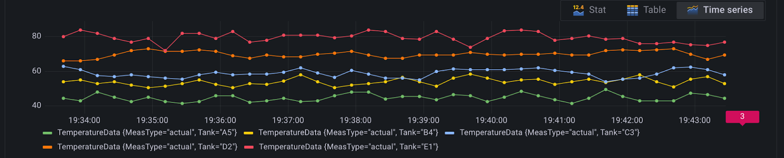
Add expressions to your Grafana Alert rule
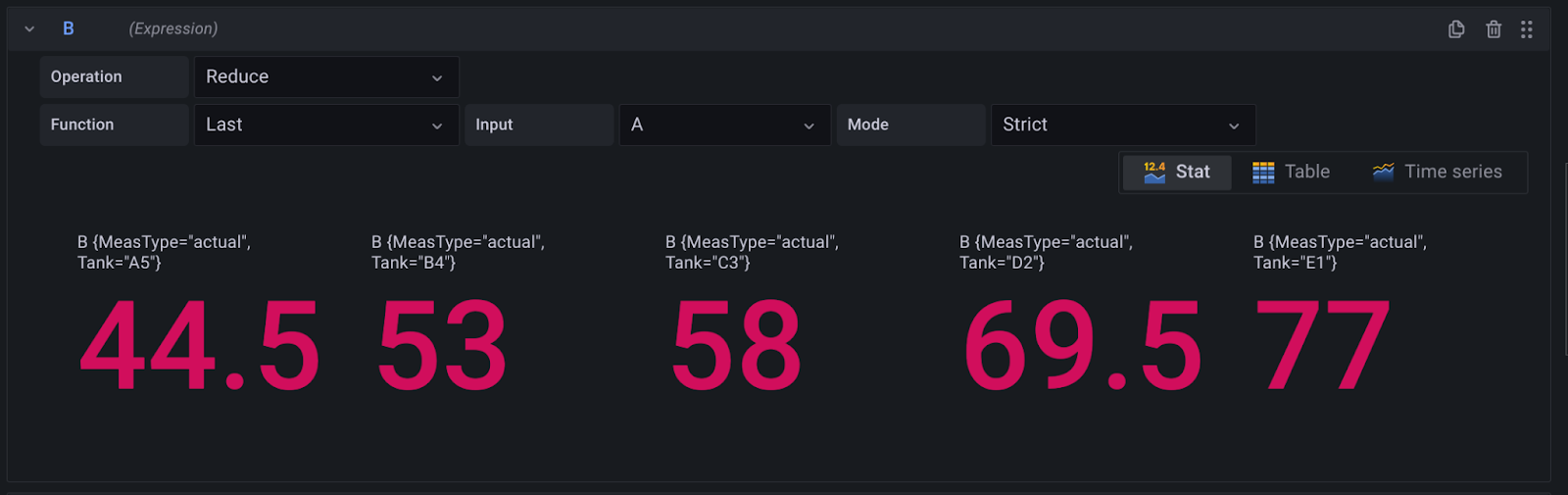
We create a Reduce expression that will reduce the time series for each tank to a single value. This gives us five distinct temperatures:
![grafana alerts from flux queries]() )
)Create a math expression to be alerted on. This is the exact same expression from example 1,
$B < 30 || $B > 60:![grafana alerts from flux queries]()
 )
)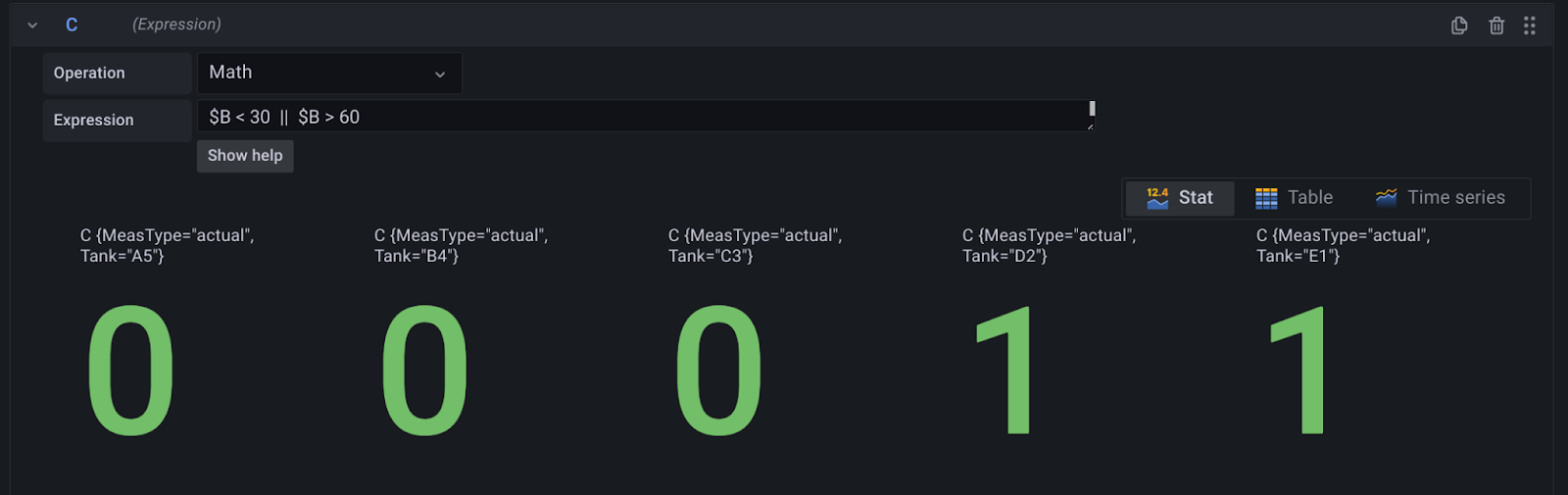
As we can see three tanks are within the acceptable thresholds while two tanks have crossed the upper boundary. This would trigger an alert for tanks D2 and E1.
Conclusion
With multidimensional alerts we can avoid repeating ourselves. But what if the scenario were even more complex? In the next and final example, we will examine how to use multidimensional alerts to create the most dynamic alerts possible.
Example 5: how to create a dynamic (multidimensional) Grafana Alert using multiple queries and multiple thresholds with Flux
For this final example let’s continue with our five fluid tanks and their five datasets.Let’s assume again that each tank has a temperature controller with a setpoint value that is stored in InfluxDB. Let’s mix things up and assume that each tank has a different setpoint, where we always need to be within 3 degrees of the setpoint.
We want to create one multidimensional alert that will cover each unique scenario for each tank, triggering an alert whenever any tank’s temperature moves beyond its unique allowable range.
To better visualize this challenge, here is a table representing our five tanks, their temperature setpoints, and their allowable range:
With Grafana Alerting, we can create a single multidimensional rule to cover all 5 tanks, and we can use Flux to compare the setpoint and actual value for each tank. In other words, one multidimensional alert can monitor 5 separate tanks, each with different setpoints and actual values, but all with one common “allowable threshold” (i.e. a temperature difference of ±3 degrees).
Add an initial Flux query to your Grafana Alert rule
Let’s begin with our data query. It is similar to our past queries, only now more complex. We must add extra functions to get our data into the proper format, including a pivot(), map(), rename(), keep(), and drop() function:
from(bucket: "HyperEncabulator")
 |> range(start: v.timeRangeStart, stop: v.timeRangeStop)
 |> filter(fn: (r) => r["_measurement"] == "TemperatureData")
 |> filter(fn: (r) => r["MeasType"] == "actual" or r["MeasType"] == "setpoint")
 |> filter(fn: (r) => r["Tank"] == "A5" or r["Tank"] == "B4" or r["Tank"] == "C3" or r["Tank"] == "D2" or r["Tank"] == "E1")
 |> filter(fn: (r) => r["_field"] == "Temperature")
 |> aggregateWindow(every: v.windowPeriod, fn: mean, createEmpty: false)
 |> pivot(rowKey:["_time"], columnKey: ["MeasType"], valueColumn: "_value")
 |> map(fn: (r) => ({ r with _value: (r.setpoint - r.actual)}))
 |> rename(columns: {_value: "difference"})
 |> keep(columns: ["_time", "difference", "Tank"])
 |> drop(columns: ["actual", "setpoint"])
 |> yield(name: "mean")
Note in the above that we are calculating the difference between the actual and the setpoint. The way Grafana parses the result from InfluxDB is that if a _value column is found, it is assumed to be a time-series. The quick workaround is to add the following rename() function:
|> rename(columns: {_value: "something"})The above query results in this time series:
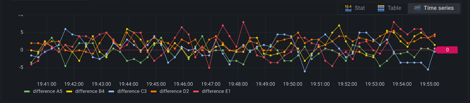
Add expressions to your Grafana Alert rule
Again, we create a Reduce expression for the above query to reduce each of the above to a single value. This value represents the temperature differential between each tank’s setpoint and its actual real-time temperature:
![grafana alerts from flux queries]()
Now we create a math expression to be alerted on. This time we will create a condition that checks if the absolute value of our reduce calculation is greater than 3,
abs($(B))>3.0:![grafana alerts from flux queries]()

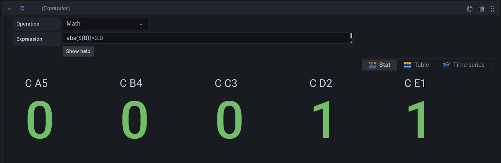
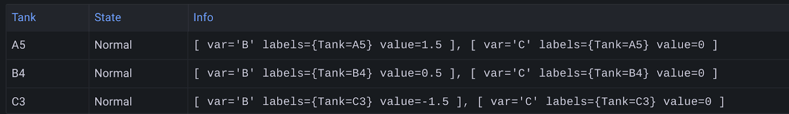
We can now see that two tanks, D2 and E1, are evaluating to true. When we preview the alert we can see that those two tanks will trigger a notification and change their state from Normal to Alerting:

Conclusion
Flux queries and Grafana Unified Alerting are a powerful combination to identify practically any alertable conditions in your dataset, or across your entire system. For more information on Grafana Alerting, visit the documentation here. For more information on the Flux query language, you can visit that documentation as well.