Continuous profiling in production: A real-world example to measure benefits and costs

Continuous profiling offers deep visibility into production environments, revealing exactly how applications consume CPU and memory. It’s the go-to observability practice for directly connecting system behavior and performance to specific lines of code. 

But when teams consider deploying continuous profiling more broadly, a common question comes up: what’s the overhead? Is it safe to run continuous profiling on my production services 24/7, or does the cost outweigh the benefits?

As a Senior Software Engineer for Pyroscope, the open source continuous profiling database, I hope to answer that question in this post. 

I’ll cover why profiling is so valuable, what “cost” really means in terms of resource usage and engineering hours, and share our own experience running continuous profiling at scale here at Grafana Labs.

Why use continuous profiling in production?

Before talking about cost, let’s explore the benefits of deploying continuous profiling in the first place.

Continuous profiling gives you a time series of where your applications spend resources, down to the line of code. That’s a different level of insight than simply knowing, for example, that a service is using 80% CPU. With continuous profiling, you see which functions and which requests are responsible for that 80%. That, in turn, lets you pinpoint root causes without needing to reproduce the issue in staging or add new instrumentation. You can identify the highest impact fixes (or roll back with confidence), which shortens MTTR.

In a GrafanaCON 2025 talk, we explained that continuous profiling uniquely improves both sides of the ROI equation:

• Revenue/reliability: Higher throughput, lower latency, and better user experience.
• Cost: Less resource waste, lower infrastructure spend, and faster incident detection and resolution.

So the real question isn’t whether continuous profiling has overhead (it does), but whether that overhead is small and predictable enough that the optimization wins outweigh the cost.

The cost equation with continuous profiling 

When people say “overhead” in the context of continuous profiling, they usually mean the runtime impact on the application: CPU, memory, and latency. But there are also backend costs, such as storing and querying profiles, as well as human costs, meaning your team’s time. 

Let’s dig into some of these, starting with what happens on the node. 

CPU and latency overhead: within a few percentage points

A lot of the hesitation around continuous profiling and overhead stems from old-school profilers that instrumented every call, wrote huge traces, or periodically halted application execution.

Pyroscope’s model is different: it relies on sampling profilers, which take a stack trace 100 times per second (100 Hz). That’s enough for a good statistical picture without touching every function call.

In a recent deep-dive post on native-code profiling with eBPF, written by Grafana Labs Staff Software Engineer Oleg Kozliuk, we explored real workloads that were benchmarked with and without profiling. The impact on throughput and latency was within a few percentage points in both cases. The setup used eBPF via Alloy and Grafana Cloud Profiles, the hosted continuous profiling tool powered by Pyroscope, but the mechanics were the same: periodic stack sampling plus lightweight metadata.

In practice, CPU and latency overhead for typical configurations lands in the low single-digit percentages, often small enough that you need synthetic benchmarks to even see it.

Memory overhead: tens of megabytes, not gigabytes

Sampling profilers are designed to have very low memory overhead, usually less than 50 MB per pod.

Here’s what’s happening under the hood:

• Stack traces are sampled at ~100 Hz.
• Allocation and lock events are sampled.
• Samples are stored in memory.
• Every 15 seconds (by default), profiles are flushed to the backend.

The main memory cost is an in-process buffer, not giant in-memory flame graphs. In practice at Grafana Labs, the overhead is often so small that the profiler's memory usage is hard to see in the profile relative to the application's memory usage.

Under the hood: where does that overhead come from?

To understand why overhead is low (and what can make it higher), it helps to look at the profiler’s control loop.

1. Sampling loop

At the heart of most continuous profilers:

• A timer fires at a fixed rate (e.g., 100 Hz).
• The profiler captures the current call stack (and maybe some metadata).
• The stack trace becomes a sample.

This step is intentionally lightweight:

• It captures stack traces, not whole heaps or object graphs.
• It avoids blocking your critical path as much as possible.

2. In-process aggregation and buffering

Instead of streaming each sample individually, Pyroscope clients:

• Aggregate samples into compact structures.
• Buffer them in memory.
• Flush them every 15 seconds (by default) to the backend.

Multiple threads are used for uploads, but the guiding principle of Pyroscope clients is to never cause the user application to crash: fail by dropping profiles, not by hurting your application. 

3. Language and profiler differences

Overhead also depends on how you collect data:

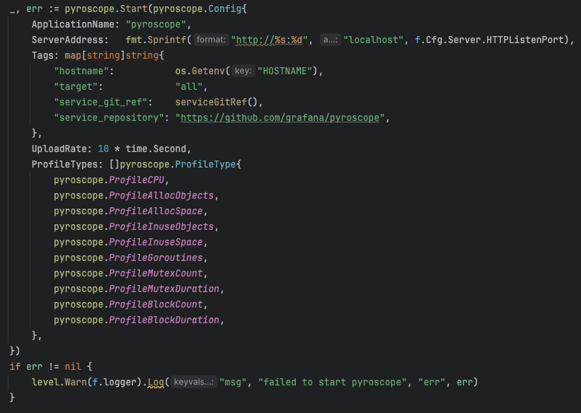
• Go: Uses Go’s built-in sampling profiler (and sometimes eBPF). Note there are push (via SDK) and pull (via Alloy’s pyroscope.scrape component) options for sending profiles to Pyroscope.
• Java: Uses AsyncProfiler or Java Flight Recorder via the Pyroscope Java agent (in the JVM process), or auto-instrumentation using Alloy's pyroscope.java component externally attaching to a running JVM using AsyncProfiler.
• .NET, Python, Ruby, Node.js, Rust: Use runtime profilers or eBPF-based approaches depending on platform.
• eBPF/system-wide: Pyroscope’s eBPF integration (via Alloy and pyroscope.ebpf) hooks perf events at the kernel level to sample stacks across processes without changing application code.

Each has different characteristics, but they share the same philosophy: sampling, not deep instrumentation.

What actually drives the cost?

Even within a single language, overhead varies. The main profiling knobs are:

Sampling rate

• Higher frequency (e.g., 200 Hz) → better resolution, more CPU overhead.
• Lower frequency (e.g., 50 Hz) → less overhead, coarser view.

The default 100 Hz works well for most teams. If you’re extremely latency-sensitive, you can reduce rates for specific services.

Profile types

More profile types = more work:

• CPU profiles are the cheapest and most common.
• Allocation/heap profiles add bookkeeping.
• Mutex/block/goroutine profiles add lock and scheduling data.

At Grafana Labs, we often run with multiple profile types enabled by default: CPU, allocations, goroutines, mutex, block, and still see per-pod memory usage stay below ~50 MB.

If you’re cost-sensitive:

• Start with CPU-only.
• Turn on additional profile types in targeted experiments (a subset of services or a specific namespace).

Workload characteristics

Some workloads are trickier to profile:

• Very short-lived tasks (sub-millisecond) can be hard to sample.
• High-churn workloads (many short connections/processes) create more sampling and aggregation work.
• Highly optimized native code (e.g., vectorized DB kernels) may be more sensitive to any extra overhead.

The good news is you can measure this in your own environment with a simple method: run a representative load test with profiling off vs. on and compare latency and throughput.

Backend and storage costs: why the server also matters

So far we’ve focused on application overhead, but continuous profiling also has a database backend like Pyroscope or Grafana Cloud Profiles.

Here the cost is storage and query performance as you scale.

Pyroscope shares architecture patterns with systems like Loki, Mimir, and Tempo (sharded, horizontally scalable, block-based storage), so it inherits the same profiling, compaction, and query-optimization work.

For users, that means:

• Lower storage cost per unit of profiling data.
• Faster queries over long time ranges.
• Predictable performance as you add services and tenants.

How to do your own “overhead reality check” with Pyroscope

1. Pick a canary + steady load
   • Choose a representative, non-critical service.
   • Put it under stable traffic (production during a quiet window or fixed-load test).
2. Enable your profiler just there
   • Enable the profiler with CPU-only and default sampling (e.g., 100 Hz).
   • Optionally, tag it (e.g., profiling=canary) so you can filter later.
3. Watch your normal metrics
   Compare profiled vs. unprofiled pods of the same service:
   • CPU per pod
   • p95/p99 latency
   • Error rate
4. This gives you a first-pass “profiling ≈ X% CPU / Y ms” answer.
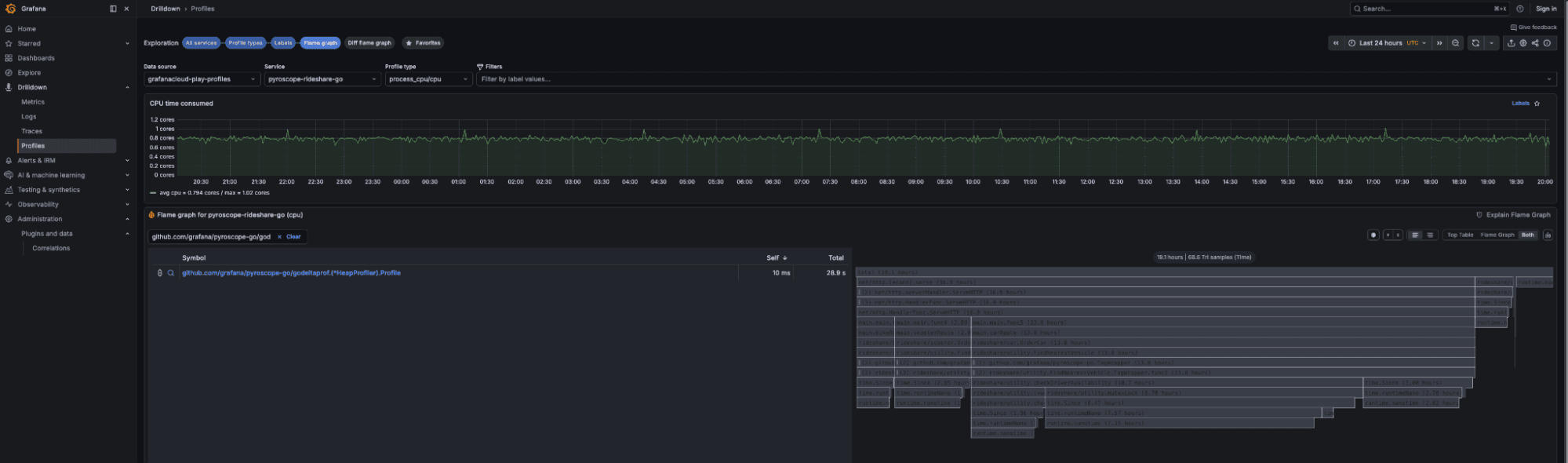
5. Use Pyroscope to see profiler cost
   In Pyroscope:
   • Filter to the canary.
   • Open a CPU flame graph.
   • Search for profiler frames (pprof, async-profiler, jfr, etc.).
6. The percentage of samples in those frames ≈ profiler overhead (e.g., 2% of samples ≈ ~2% CPU).

When someone asks, “Is this cost-effective in production?” you won’t be guessing — you’ll have numbers from your own environment, measured by Pyroscope.

Bringing it all together

If you’ve had bad experiences with heavy profilers, skepticism is reasonable. But modern sampling profilers, in combination with Pyroscope, tell a different story:

• Memory overhead is typically <50 MB per pod, even with multiple profile types enabled.
• CPU and latency overhead in realistic benchmarks sits in the low single-digit percentage range.

In other words, you’re trading a small, predictable overhead for the ability to:

• Catch performance regressions before they hit customers.
• Make expensive infrastructure actually earn its keep.
• Answer “where is the CPU going?” in minutes instead of days.

That’s a tradeoff we’re happy to make across all of our own production workloads at Grafana Labs, and one that more and more teams are adopting as continuous profiling moves from nice-to-have to a standard observability pillar.

To learn more, please check out our Pyroscope documentation or reach out in the #pyroscope channel in our Grafana Labs Community Slack.