
A beginner’s guide to distributed tracing and how it can increase an application’s performance
Most people are instrumenting their applications, with logs being an easy first step into the observability world, followed by metrics.
Tracing lags behind these two and is maybe a little less used than other observability patterns.
We hope to change that.
Grafana Labs recently launched an easy-to-operate, high-scale, and cost-effective distributed tracing backend: Grafana Tempo. Tempo’s only dependency is object storage. Unlike other tracing backends, Tempo can hit massive scale without a difficult-to-manage Elasticsearch or Cassandra cluster. Tempo supports search solely via trace id; logs and Prometheus exemplars can be used to find traces effectively. In short, Tempo allows us to scale tracing as far as possible with less operational cost and complexity than ever before.
On Feb. 4, Grafana Labs Senior Backend Developer Joe Elliott will be hosting a webinar all about getting started with tracing with Tempo, and the Grafana integrations that seamlessly link your metrics, logs, and traces. You can register for the event here.
In the meantime, here’s an outline of the basics around distributed tracing. Along with explaining how tracing works, we also address why developers should work to incorporate distributed tracing into their applications and how investing the money and time to build the infrastructure and install the code for tracing can increase an application’s performance.
Observability basics: metrics and logs
Before we discuss tracing, let’s start by reviewing metrics and logs, which will help set the stage for what tracing could do for you and what hole it could fill.

The great strength of metrics? They’re aggregatable. They are aggregations of the behavior of our systems. Therefore, they are easy to query, and they are cheap to store. They are often stored as time series data, which is just a timestamp and a value. And that compresses very nicely, which makes it very easy to store and query them very quickly.

Cardinality, however, plays a major factor when discussing metrics, especially when there is too much of it. Cardinality explosions occur when too many metrics or labels are added, which, in turn, increases the cost of storage, the size of the index, and the query speed. In short, you’ve defeated the point of metrics.
Metrics are meant to be simple. We have small indexes that cover enormous amounts of data, and small amounts of data that cover an enormous range of behavior in our applications. For that reason, we want metrics to be aggregated. That is the point of metrics; that is why we store them and query them.

In addition to metrics, logs are an important form of instrumentation that helps assess the health of a service.
Grafana Labs uses Grafana Loki, a horizontally scalable, highly available, multi-tenant log aggregation system inspired by Prometheus. It is designed to be very cost-effective and easy to operate. It does not index the contents of the logs, but rather a set of labels for each log stream.
The query and logs shown above are from one of Grafana Labs’ applications. Users can look at a single service and query all the logs that are occurring within the service. They can also see a series’ “events.” Or they could query across a lot of services and sometimes grab a whole set of services, looking for specific errors or errors in general.
But in all cases, logs are a series of events that occur sequentially in time.
One of the most common patterns is that someone gets an alert or someone may notice something is wrong with a metric on a dashboard at an overview aggregation level. Often the next steps would be to write some queries to roughly find out what’s wrong in the metrics engine and what services are having issues. Then logs can be used to retrieve more detailed information about what’s wrong with that specific service.
While metrics and logs can work together to pinpoint a problem, they both lack important elements. Metrics, though good for aggregations, lack fine-grained information. Logs are good at revealing what happened sequentially in an application, or maybe even across applications, but they don’t show how a single request perhaps behaves inside of a service.
It’s difficult to track a request to know why a request is slow. Logs will tell us why a service is having issues, but maybe not why a given request is having issues.
Why distributed tracing?

Tracing is the answer to all of this.
Distributed tracing is a way to track a single request and log a single request as it crosses through all of the services in your infrastructure.
The slide above highlights a Prometheus query that’s hitting Cortex, the scalable Prometheus project that has advanced to incubation within CNCF. The request was passed down through four different services in about 18 milliseconds, and there is a lot of detail about how the request is handled. If this request took 5 seconds or 10 seconds or something awful, then the trace could tell us exactly where it spent those 10 seconds — and perhaps why it spent time in certain areas — to help us understand what’s going on in an infrastructure or how to fix a problem.
In tracing, a span is a representation of a unit of work in a given application, and they are represented by all the horizontal bars in the query above. If we made a query to a backend, to a database, or to a caching server, we could wrap those in spans to get information about how long each of those pieces took.
Spans are related to each other in a handful of different ways, but primarily by a parent-child relationship. So in the Cortex query, there are two related spans in which promqlEval is the parent and promqlPrepare is a child. This relationship is how our tracing backend is able to take all these spans and actually rebuild them into a single trace and return that trace when we ask for it.
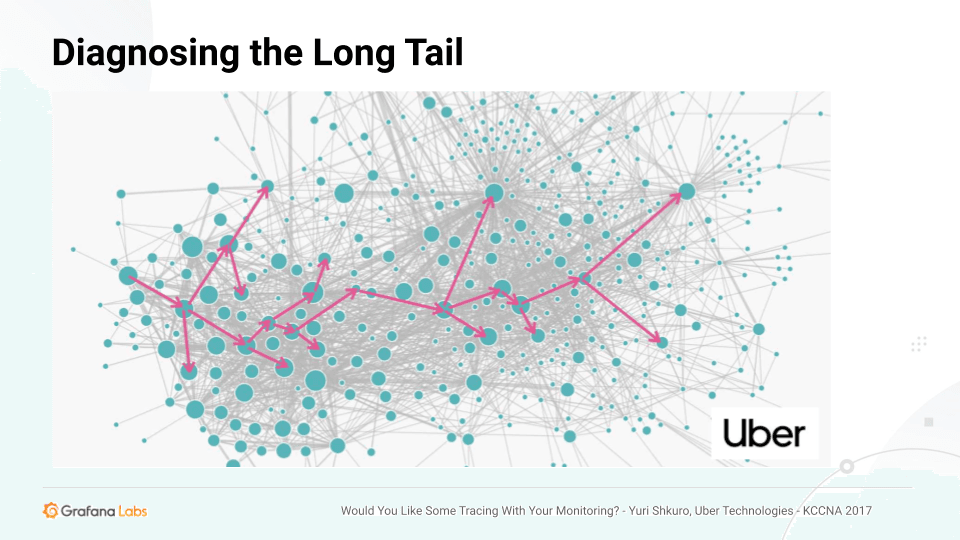
The big win with distributed tracing is diagnosing the long tail.
When there is a set of queries hitting an especially complicated infrastructure, for example, the P50 could be normal and the P90 could be 15 milliseconds, but the P99 could be 5 seconds — which needs to be reduced. All the metrics could look okay except for this elevated P99. The cache and the database could be responding quickly. So why are some queries very long?
Tracing is a great way to diagnose that issue. You can find these longer queries, go into the trace and really dig into the exact behavior of the query or the requests so that you can determine where to spend your development efforts.
The above example shows a very complex microservices infrastructure that existed at Uber, which developed the popular open source end-to-end distributed tracing system Jaeger. But while microservices lend themselves to leveraging tracing to determine and understand how requests are passed through services and gain information about them, tracing is effective in monoliths as well.
Monoliths can be very complicated. They can have extremely complex modules, and a given query can pass through hundreds or thousands of them just like a given query can pass through hundreds or thousands of services. Understanding the way an exact query was executed in a monolith can be very difficult, but tracing can shed light on that as well. So distributed tracing is very valuable in a monolith or a microservices world, or a hybrid of both.
Context propagation

Whether there are 10 services or 100 services, they’re all receiving requests, and they’re all building spans that describe what the request is doing. All these spans are then sent or streamed to the backend independently. So the question becomes, how do we rebuild those?
That’s where context propagation comes in.
Developers can purposefully propagate context through an HTTP request to perform functions such as tracing. That context is passed down through all the functions as you execute your request and then should also be passed to the next set of services.
This context is where tracing information is buried, such as the trace ID or the parent span ID, which help rebuild the spans when we send them to the backend. So every time you create a span, it’s going to check the context, and it’s going to see if there’s an existing span or any existing trace. If there is, it will become a part of that trace. It will use that trace ID, and that will allow the backend to rebuild.
Between services, the context will be attached to HTTP headers or gRPC headers and metadata about our query to the backend. Then that metadata will propagate the trace across services. So in-service we’re using an in-memory context object. Cross-service, we’re using headers or other metadata associated with our query.
How does tracing work?
You can watch a demo here of how to take a simple application, instrument it for tracing, build spans, and offload those traces to a Jaeger backend. In this video, you’ll also see the workflow of how to run a typical Loki search, retrieve the trace from Jaeger, and view the trace in Grafana.
There’s also a deeper dive into spans and how attaching metadata such as logs, events, or tags, can provide more information about what is going on in the request as it passes down through your architecture.
You can clone the repo for the demo on Github and use it as a reference.
Be sure to tune in to the Feb. 4 webinar on how to get started with Tempo for more on how to get the most out of tracing.
You can also get free open-beta access to Tempo on Grafana Cloud. We have new free and paid Grafana Cloud plans to suit every use case — sign up for free now.

