Important: This documentation is about an older version. It's relevant only to the release noted, many of the features and functions have been updated or replaced. Please view the current version.

Documentation Grafana documentation Panels and visualizations Query and transform data Transform data

Transform data

Transformations are a powerful way to manipulate data returned by a query before the system applies a visualization. Using transformations, you can:

• Rename fields
• Join time series data
• Perform mathematical operations across queries
• Use the output of one transformation as the input to another transformation

For users that rely on multiple views of the same dataset, transformations offer an efficient method of creating and maintaining numerous dashboards.

You can also use the output of one transformation as the input to another transformation, which results in a performance gain.

Sometimes the system cannot graph transformed data. When that happens, click the Table view toggle above the visualization to switch to a table view of the data. This can help you understand the final result of your transformations.

Transformation types

Grafana provides a number of ways that you can transform data. For a complete list of transformations, refer to Transformation functions.

Order of transformations

When there are multiple transformations, Grafana applies them in the order they are listed. Each transformation creates a result set that then passes on to the next transformation in the processing pipeline.

The order in which Grafana applies transformations directly impacts the results. For example, if you use a Reduce transformation to condense all the results of one column into a single value, then you can only apply transformations to that single value.

Add a transformation function to data

The following steps guide you in adding a transformation to data. This documentation does not include steps for each type of transformation. For a complete list of transformations, refer to Transformation functions.

1. Navigate to the panel where you want to add one or more transformations.
2. Click the panel title and then click Edit.
3. Click the Transform tab.
4. Click a transformation. A transformation row appears where you configure the transformation options. For more information about how to configure a transformation, refer to Transformation functions. For information about available calculations, refer to Calculation types.
5. To apply another transformation, click Add transformation. This transformation acts on the result set returned by the previous transformation.

Debug a transformation

To see the input and the output result sets of the transformation, click the bug icon on the right side of the transformation row.

The input and output results sets can help you debug a transformation.

Delete a transformation

We recommend that you remove transformations that you don’t need. When you delete a transformation, you remove the data from the visualization.

Before you begin:

• Identify all dashboards that rely on the transformation and inform impacted dashboard users.

To delete a transformation:

1. Open a panel for editing.
2. Click the Transform tab.
3. Click the trash icon next to the transformation you want to delete.

Transformation functions

You can perform the following transformations on your data.

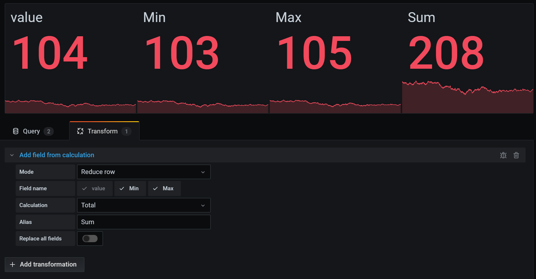
Add field from calculation

Use this transformation to add a new field calculated from two other fields. Each transformation allows you to add one new field.

• Mode - Select a mode:
  • Reduce row - Apply selected calculation on each row of selected fields independently.
  • Binary option - Apply basic math operation(sum, multiply, etc) on values in a single row from two selected fields.
• Field name - Select the names of fields you want to use in the calculation for the new field.
• Calculation - If you select Reduce row mode, then the Calculation field appears. Click in the field to see a list of calculation choices you can use to create the new field. For information about available calculations, refer to Calculation types.
• Operation - If you select Binary option mode, then the Operation fields appear. These fields allow you to do basic math operations on values in a single row from two selected fields. You can also use numerical values for binary operations.
• Alias - (Optional) Enter the name of your new field. If you leave this blank, then the field will be named to match the calculation.
• Replace all fields - (Optional) Select this option if you want to hide all other fields and display only your calculated field in the visualization.

In the example below, I added two fields together and named them Sum.

Concatenate fields

This transformation combines all fields from all frames into one result. Consider:

Query A:

Query B:

After you concatenate the fields, the data frame would be:

Config from query results

This transformation allow you to select one query and from it extract standard options like Min, Max, Unit and Thresholds and apply it to other query results. This enables dynamic query driven visualization configuration.

If you want to extract a unique config for every row in the config query result then try the rows to fields transformation.

Options

• Config query: Select the query that returns the data you want to use as configuration.
• Apply to: Select what fields or series to apply the configuration to.
• Apply to options: Usually a field type or field name regex depending on what option you selected in Apply to.

Convert field type

This transformation changes the field type of the specified field.

• Field - Select from available fields
• as - Select the FieldType to convert to
  • Numeric - attempts to make the values numbers
  • String - will make the values strings
  • Time - attempts to parse the values as time
    • Will show an option to specify a DateFormat as input by a string like yyyy-mm-dd or DD MM YYYY hh:mm:ss
  • Boolean - will make the values booleans

For example the following query could be modified by selecting the time field, as Time, and Date Format as YYYY.

The result:

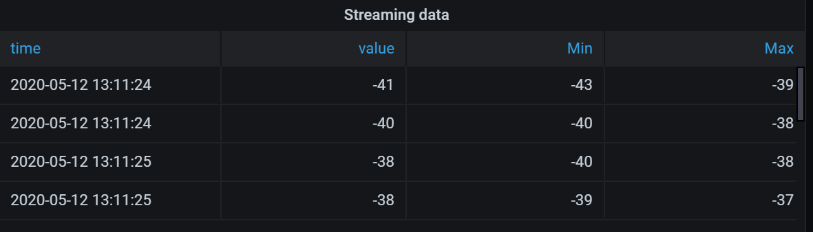
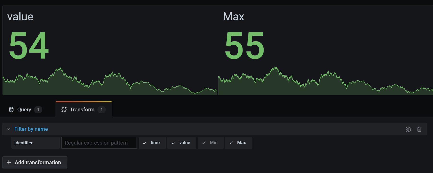
Filter data by name

Use this transformation to remove portions of the query results.

Grafana displays the Identifier field, followed by the fields returned by your query.

You can apply filters in one of two ways:

• Enter a regex expression.
• Click a field to toggle filtering on that field. Filtered fields are displayed with dark gray text, unfiltered fields have white text.

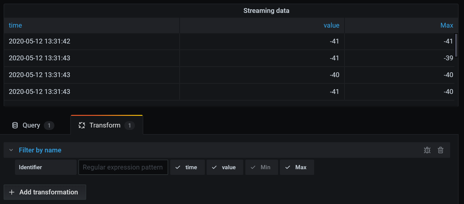
In the example below, I removed the Min field from the results.

Here is the original query table. (This is streaming data, so numbers change over time and between screenshots.)

Here is the table after I applied the transformation to remove the Min field.

Here is the same query using a Stat visualization.

Filter data by query

Use this transformation in panels that have multiple queries, if you want to hide one or more of the queries.

Grafana displays the query identification letters in dark gray text. Click a query identifier to toggle filtering. If the query letter is white, then the results are displayed. If the query letter is dark, then the results are hidden.

In the example below, the panel has three queries (A, B, C). I removed the B query from the visualization.

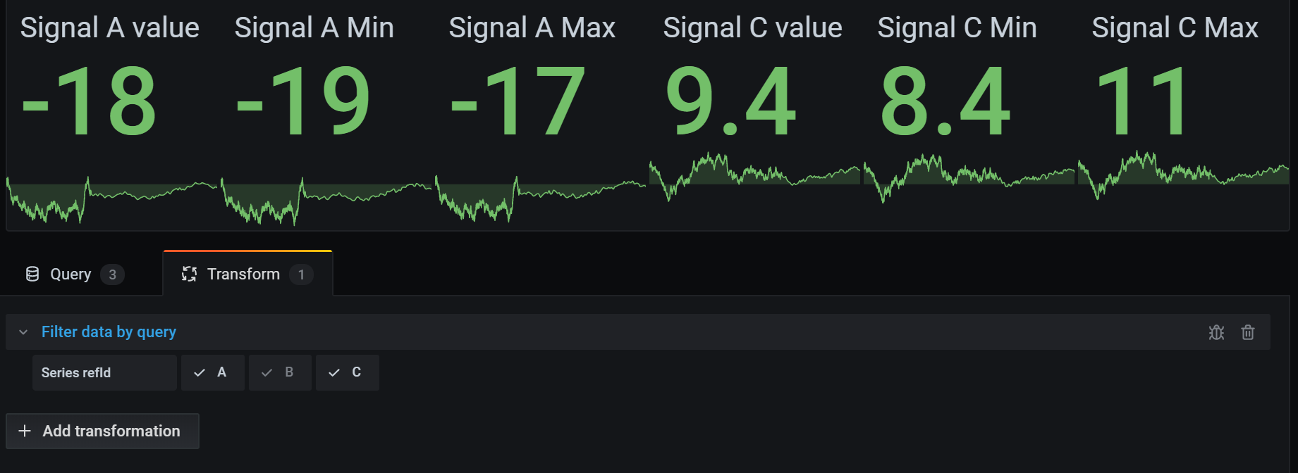
Note: This transformation is not available for Graphite because this data source does not support correlating returned data with queries.

Filter data by value

This transformation allows you to filter your data directly in Grafana and remove some data points from your query result. You have the option to include or exclude data that match one or more conditions you define. The conditions are applied on a selected field.

This transformation is very useful if your data source does not natively filter by values. You might also use this to narrow values to display if you are using a shared query.

The available conditions for all fields are:

• Regex: Match a regex expression
• Is Null: Match if the value is null
• Is Not Null: Match if the value is not null
• Equal: Match if the value is equal to the specified value
• Different: match if the value is different than the specified value

The available conditions for number fields are:

• Greater: Match if the value is greater than the specified value
• Lower: Match if the value is lower than the specified value
• Greater or equal: Match if the value is greater or equal
• Lower or equal: Match if the value is lower or equal
• Range: Match a range between a specified minimum and maximum, min and max included

Consider the following data set:

If you Include the data points that have a temperature below 30°C, the configuration will look as follows:

• Filter Type: Include
• Condition: Rows where Temperature matches Lower Than 30

And you will get the following result, where only the temperatures below 30°C are included:

You can add more than one condition to the filter. For example, you might want to include the data only if the altitude is greater than 100. To do so, add that condition to the following configuration:

• Filter type: Include rows that Match All conditions
• Condition 1: Rows where Temperature matches Lower than 30
• Condition 2: Rows where Altitude matches Greater than 100

When you have more than one condition, you can choose if you want the action (include / exclude) to be applied on rows that Match all conditions or Match any of the conditions you added.

In the example above we chose Match all because we wanted to include the rows that have a temperature lower than 30 AND an altitude higher than 100. If we wanted to include the rows that have a temperature lower than 30 OR an altitude higher than 100 instead, then we would select Match any. This would include the first row in the original data, which has a temperature of 32°C (does not match the first condition) but an altitude of 101 (which matches the second condition), so it is included.

Conditions that are invalid or incompletely configured are ignored.

Group by

This transformation groups the data by a specified field (column) value and processes calculations on each group. Click to see a list of calculation choices. For information about available calculations, refer to Calculation types.

Here’s an example of original data.

This transformation goes in two steps. First you specify one or multiple fields to group the data by. This will group all the same values of those fields together, as if you sorted them. For instance if we group by the Server ID field, then it would group the data this way:

All rows with the same value of Server ID are grouped together.

After choosing which field you want to group your data by, you can add various calculations on the other fields, and apply the calculation to each group of rows. For instance, we could want to calculate the average CPU temperature for each of those servers. So we can add the mean calculation applied on the CPU Temperature field to get the following:

And we can add more than one calculation. For instance:

• For field Time, we can calculate the Last value, to know when the last data point was received for each server
• For field Server Status, we can calculate the Last value to know what is the last state value for each server
• For field Temperature, we can also calculate the Last value to know what is the latest monitored temperature for each server

We would then get :

This transformation enables you to extract key information from your time series and display it in a convenient way.

Join by field

Use this transformation to join multiple results into a single table. This is especially useful for converting multiple time series results into a single wide table with a shared time field.

Inner join

An inner join merges data from multiple tables where all tables share the same value from the selected field. This type of join excludes data where values do not match in every result.

Use this transformation to combine the results from multiple queries (combining on a passed join field or the first time column) into one result, and drop rows where a successful join cannot occur.

In the following example, two queries return table data. It is visualized as two separate tables before applying the inner join transformation.

Query A:

Query B:

The result after applying the inner join transformation looks like the following:

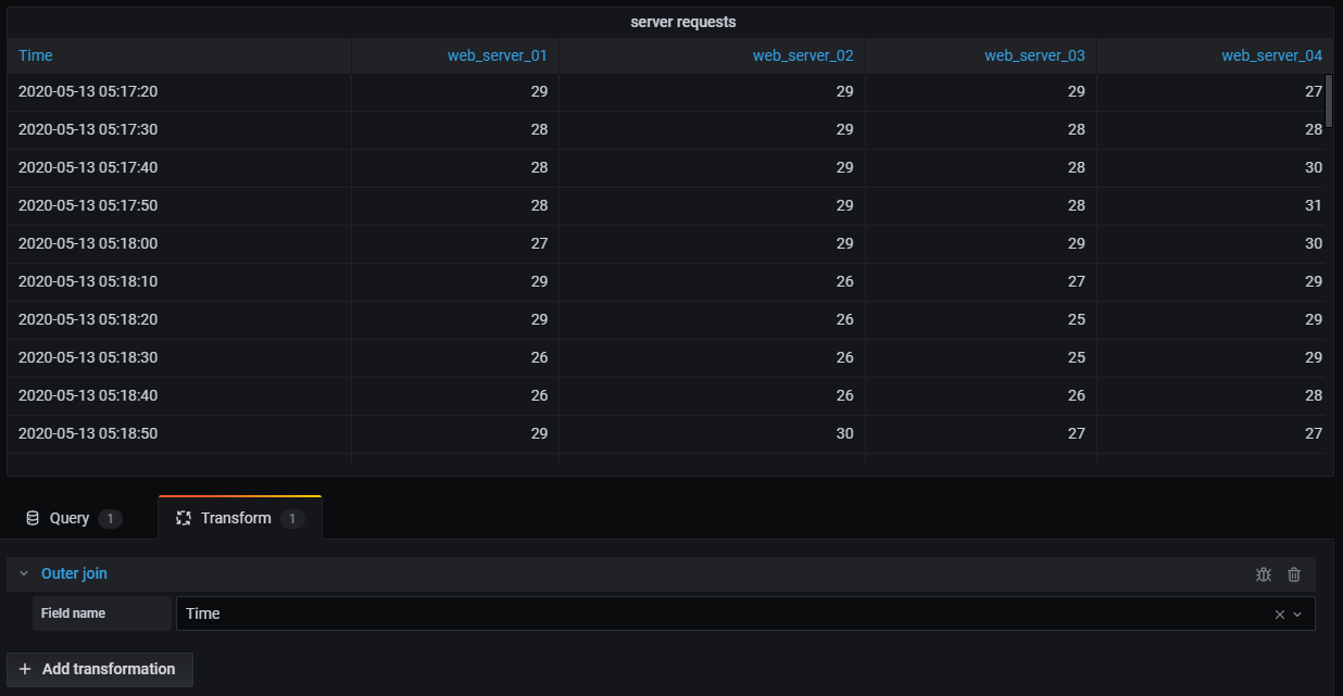
Outer join

An outer join includes all data from an inner join and rows where values do not match in every input. While the inner join joins Query A and Query B on the time field, the outer join includes all rows that don’t match on the time field.

In the following example, two queries return table data. It is visualized as two tables before applying the outer join transformation.

Query A:

Query B:

The result after applying the outer join transformation looks like the following:

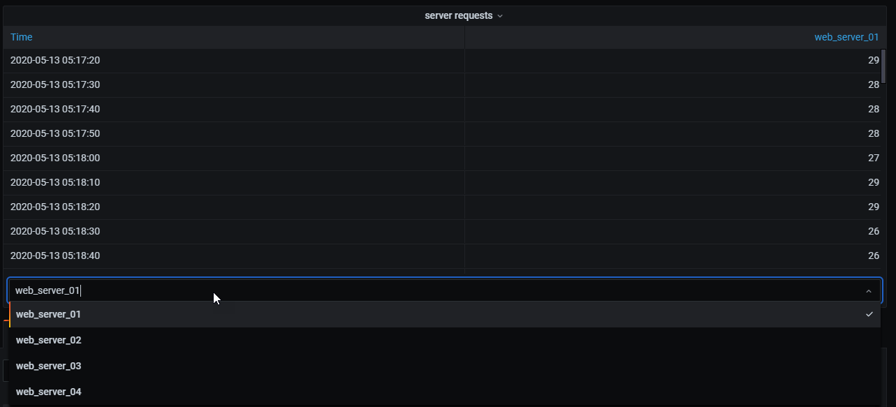
In the following example, a template query displays time series data from multiple servers in a table visualization. The results of only one query can be viewed at a time.

I applied a transformation to join the query results using the time field. Now I can run calculations, combine, and organize the results in this new table.

Labels to fields

This transformation changes time series results that include labels or tags into a table where each label keys and values are included in the table result. The labels can be displayed either as columns or as row values.

Given a query result of two time series:

• Series 1: labels Server=Server A, Datacenter=EU
• Series 2: labels Server=Server B, Datacenter=EU

In “Columns” mode, the result looks like this:

In “Rows” mode, the result has a table for each series and show each label value like this:

Value field name

If you selected Server as the Value field name, then you would get one field for every value of the Server label.

Merging behavior

The labels to fields transformer is internally two separate transformations. The first acts on single series and extracts labels to fields. The second is the merge transformation that joins all the results into a single table. The merge transformation tries to join on all matching fields. This merge step is required and cannot be turned off.

To illustrate this, here is an example where you have two queries that return time series with no overlapping labels.

• Series 1: labels Server=ServerA
• Series 2: labels Datacenter=EU

This will first result in these two tables:

After merge:

Merge

Use this transformation to combine the result from multiple queries into one single result. This is helpful when using the table panel visualization. Values that can be merged are combined into the same row. Values are mergeable if the shared fields contain the same data. For information, refer to Table panel.

In the example below, we have two queries returning table data. It is visualized as two separate tables before applying the transformation.

Query A:

Query B:

Here is the result after applying the Merge transformation.

Organize fields

Use this transformation to rename, reorder, or hide fields returned by the query.

Note: This transformation only works in panels with a single query. If your panel has multiple queries, then you must either apply an Outer join transformation or remove the extra queries.

Grafana displays a list of fields returned by the query. You can:

• Change field order by hovering your cursor over a field. The cursor turns into a hand and then you can drag the field to its new place.
• Hide or show a field by clicking the eye icon next to the field name.
• Rename fields by typing a new name in the Rename box.

In the example below, I hid the value field and renamed Max and Min.

Partition by values

This transformation can help eliminate the need for multiple queries to the same datasource with different WHERE clauses when graphing multiple series. Consider a metrics SQL table with the following data:

Prior to v9.3, if you wanted to plot a red trendline for US and a blue one for EU in the same TimeSeries panel, you would likely have to split this into two queries:

SELECT Time, Value FROM metrics WHERE Time > '2022-10-20' AND Region='US'
SELECT Time, Value FROM metrics WHERE Time > '2022-10-20' AND Region='EU'

This also requires you to know ahead of time which regions actually exist in the metrics table.

With the Partition by values transformer, you can now issue a single query and split the results by unique values in one or more columns (fields) of your choosing. The following example uses Region.

SELECT Time, Region, Value FROM metrics WHERE Time > '2022-10-20'

Reduce

The Reduce transformation applies a calculation to each field in the frame and return a single value. Time fields are removed when applying this transformation.

Consider the input:

Query A:

Query B:

The reduce transformer has two modes:

• Series to rows - Creates a row for each field and a column for each calculation.
• Reduce fields - Keeps the existing frame structure, but collapses each field into a single value.

For example, if you used the First and Last calculation with a Series to rows transformation, then the result would be:

The Reduce fields with the Last calculation, results in two frames, each with one row:

Query A:

Query B:

Rename by regex

Use this transformation to rename parts of the query results using a regular expression and replacement pattern.

You can specify a regular expression, which is only applied to matches, along with a replacement pattern that support back references. For example, let’s imagine you’re visualizing CPU usage per host and you want to remove the domain name. You could set the regex to ([^\.]+)\..+ and the replacement pattern to $1, web-01.example.com would become web-01.

In the following example, we are stripping the prefix from event types. In the before image, you can see everything is prefixed with system.

With the transformation applied, you can see we are left with just the remainder of the string.

Rows to fields

The rows to fields transformation converts rows into separate fields. This can be useful as fields can be styled and configured individually. It can also use additional fields as sources for dynamic field configuration or map them to field labels. The additional labels can then be used to define better display names for the resulting fields.

This transformation includes a field table which lists all fields in the data returned by the config query. This table gives you control over what field should be mapped to each config property (the *Use as** option). You can also choose which value to select if there are multiple rows in the returned data.

This transformation requires:

• One field to use as the source of field names.

  By default, the transform uses the first string field as the source. You can override this default setting by selecting Field name in the Use as column for the field you want to use instead.

• One field to use as the source of values.

  By default, the transform uses the first number field as the source. But you can override this default setting by selecting Field value in the Use as column for the field you want to use instead.

Useful when visualizing data in:

• Gauge
• Stat
• Pie chart

Map extra fields to labels

If a field does not map to config property Grafana will automatically use it as source for a label on the output field-

Example:

Output:

The extra labels can now be used in the field display name provide more complete field names.

If you want to extract config from one query and appply it to another you should use the config from query results transformation.

Example

Input:

Output:

As you can see each row in the source data becomes a separate field. Each field now also has a max config option set. Options like Min, Max, Unit and Thresholds are all part of field configuration and if set like this will be used by the visualization instead of any options manually configured in the panel editor options pane.

Prepare time series

Note: This transformation is available in Grafana 7.5.10+ and Grafana 8.0.6+.

Prepare time series transformation is useful when a data source returns time series data in a format that isn’t supported by the panel you want to use. For more information about data frame formats, refer to Data frames.

This transformation helps you resolve this issue by converting the time series data from either the wide format to the long format or the other way around.

Select the Multi-frame time series option to transform the time series data frame from the wide to the long format.

Select the Wide time series option to transform the time series data frame from the long to the wide format.

Series to rows

Note: This transformation is available in Grafana 7.1+.

Use this transformation to combine the result from multiple time series data queries into one single result. This is helpful when using the table panel visualization.

The result from this transformation will contain three columns: Time, Metric, and Value. The Metric column is added so you easily can see from which query the metric originates from. Customize this value by defining Label on the source query.

In the example below, we have two queries returning time series data. It is visualized as two separate tables before applying the transformation.

Query A:

Query B:

Here is the result after applying the Series to rows transformation.

Sort by

This transformation will sort each frame by the configured field, When reverse is checked, the values will return in the opposite order.

Limit

Use this transformation to limit the number of rows displayed.

In the example below, we have the following response from the data source:

Here is the result after adding a Limit transformation with a value of ‘3’: