Documentation Plugins Databricks data source Query editor

Databricks query editor

Grafana provides a query editor for Databricks data source, which is located on the Explore page. You can also access the query editor from a dashboard panel. Click the menu in the upper right of the panel and select Edit.

This document explains querying specific to the Databricks data source. For general documentation on querying data sources in Grafana, refer to Query and transform data. For options and functions common to all query editors, refer to Query editors.

The Databricks query editor has two modes:

• Builder mode
• Code mode

To switch between the editor modes, select the corresponding Builder and Code tabs in the upper right.

To run a query, select Run query in the upper right of the editor.

In addition to writing queries, the query editor also allows you to create and use:

• Macros
• Annotations

Builder mode

Builder mode allows you to build queries using a visual interface. This mode is great for users who prefer a guided query experience or are just getting started with Databricks SQL, which is based on Apache Spark SQL. For more information on Databricks SQL, refer to the SQL language reference in the Databricks documentation.

The following components will help you build a Databricks SQL query:

• Format - Select a format response from the drop-down for the Databricks query. The default is Table. Refer to Table queries and Time series queries for more information and examples. If you select the Time series format option, you must include a time column.
• Filter - Toggle to add filters.
• Filter by column value - Optional. If you toggle Filter you can add a column to filter by from the drop-down. To filter by additional columns, click the + sign to the right of the condition drop-down. You can choose a variety of operators from the drop-down next to the condition. When multiple filters are added, use the AND or OR operators to define how conditions are evaluated. AND requires all conditions to be true, while OR requires any condition to be true. Use the second drop-down to select the filter value. To remove a filter, click the X icon next to it. If you select a date-type column, you can use macros from the operator list and choose timeFilter to insert the $\_\_timeFilter macro into your query with the selected date column.
• Group - Toggle to add a GROUP BY column.
• Group by column - Select a column to filter by from the drop-down. Click the +sign to filter by multiple columns. Click the X to remove a filter.
• Order - Toggle to add an ORDER BY statement.
• Order by - Select a column to order by from the drop-down. Select ascending (ASC) or descending (DESC) order.
• Limit - You can add an optional limit on the number of retrieved results. Default is 50.
• Preview - Toggle for a preview of the SQL query generated by the query builder. Preview is toggled on by default.
• Schema - Select a schema from the drop-down. The schema is a logical container that organizes and groups related database objects like tables, views, and functions within a catalog. It forms part of Databricks’ three-level namespace hierarchy: catalog.schema.table.
• Table - Select a table from the drop-down. Table selection is dependent on schema.
• Column - Select a column from the drop-down. A column is a named field within a table that holds data of a specific data type. You can select multiple columns.
• Aggregation Optional. Select an aggregation type from the drop-down. Databricks SQL supports an extensive variety of aggregation types,including specialized aggregations. You can select multiple aggregations.

Code mode

Use Code mode to build complex queries using a text editor with helpful features like syntax highlighting, autocompletion, and support for macros. This mode is ideal when you need to write subqueries, apply advanced filtering, or use SQL constructs that the visual builder may not support.

You can switch back to Builder mode, but some parts of your query, such as custom SQL, macros, or non-standard clauses, may not render correctly or be editable in the visual interface.

Unity Catalog support

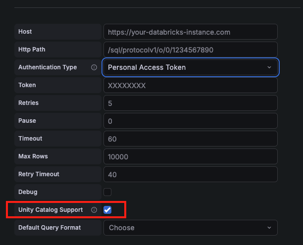
Enabling Unity Catalog support allows Grafana to connect to Databricks Unity Catalog and display available catalogs directly in the query editor. You enable Unity Catalog support when configuring the Databricks data source. When this option is enabled, the Schema drop-down is replaced with a Unity Catalog drop-down that lists all available schemas within each catalog. This enables you to query data using the full three-level namespace format: catalog.schema.table.

For more information, refer to What is Unity Catalog? in the Databricks documentation.

Enable Unity Catalog

To enable Unity Catalog support in your Databricks data source:

1. Navigate to your Databricks data source configuration page.
2. Under the connection settings, find the Unity Catalog Support checkbox.
3. Enable the checkbox to activate Unity Catalog features.
4. Click Save & Test to verify the connection.

Unity Catalog example query

Following is a basic example query using the Unity Catalog hierarchical three-level namespace:

SQL Copy

SELECT * 
FROM mycatalog.myschema.mytable
LIMIT 100;

You can also use Grafana macros and variables in your queries. For example, to filter by the dashboard time range:

SQL Copy

SELECT
  event_time AS time,
  user,
  action
FROM mycatalog.myschema.mytable
WHERE $__timeFilter(event_time)
ORDER BY event_time DESC
LIMIT 500;

Table queries

To create a Table query, set the Format option in the query editor to Table. This mode lets you to write any valid Databricks SQL query, The Table visualization then displays the results as rows and columns, exactly as returned by the query.

Example query:

SQL Copy

SELECT 
    order_date,
    customer_id,
    product_name,
    quantity,
    unit_price,
    (quantity * unit_price) AS total_amount
FROM sales.orders
WHERE order_date >= '2022-01-01'
ORDER BY order_date DESC
LIMIT 100

This query retrieves the 100 most recent orders placed on or after January 1, 2022. It returns each order’s date, customer ID, product name, quantity, unit price, and calculates a total_amount column by multiplying quantity by unit_price. Grafana displays these results as a table, allowing you to sort, filter, or transform the data directly within the panel.

Time series queries

To create a Time series query, set the Format option to Time series. Your query must include a datetime field (ideally aliased as time), which Grafana uses as the timestamp column. Grafana interprets timestamp values without an explicit time zone as UTC, and all columns except the time column are treated as value columns.

Example:

SQL Copy

SELECT
  event_time AS datetime,
  COUNT(*) AS total_events
FROM events
WHERE event_time BETWEEN $__timeFrom() AND $__timeTo()
GROUP BY event_time
ORDER BY event_time

This query returns the total number of events that occurred over time. It counts all rows in the events table for each timestamp within the Grafana dashboard’s selected time range. The macros $__timeFrom() and $__timeTo() automatically substitute the start and end times from the dashboard’s time picker.

Multi-line time series

To create multi-line time series, the query must return at least three fields in the following order:

• field 1: datetime field with an alias of time
• field 2: value to group by
• field 3+: the metric values

Example:

SQL Copy

SELECT log_time AS time, machine_group, avg(disk_free) AS avg_disk_free
FROM mgbench.logs1
GROUP BY machine_group, log_time
ORDER BY log_time

This query returns the average disk space available (avg_disk_free) over time for each machine_group. Grafana uses the time column for the x-axis, and creates a separate line for each distinct machine_group value. Each line shows how the average free disk space changes over time for that specific group.

Macros

The Databricks data source includes built-in macros that simplify working with time-based queries. These macros automatically expand into SQL expressions when your queries run, enabling you to build dynamic queries that respond to dashboard time ranges and interval controls.

Use these macros to filter data by the dashboard’s selected time range, group results by dynamic time intervals, and create time series visualizations that automatically adapt to different time periods. Just include the macro syntax in your SQL query, and Grafana handles the rest by replacing each macro with the appropriate SQL code based on your current dashboard settings.

$__interval_long macro

The $__interval_long macro converts Grafana’s dashboard interval into a Spark SQL-compatible INTERVAL format, making it easy to use with Spark SQL window functions.

Example query:

SQL Copy

SELECT window.start, avg(aggqueue) FROM a17
GROUP BY window(_time, '$__interval_long')

This query calculates the average of aggqueue values grouped into time windows. The window() function creates time-based buckets using the _time column, with the bucket size determined by the $__interval_long macro. The window size automatically adjusts based on your dashboard’s interval setting, allowing the same query to work across different time ranges and zoom levels.

Expanded query (when the dashboard interval is set to 2 minutes):

SQL Copy

SELECT window.start, avg(aggqueue) FROM a17
GROUP BY window(_time, '2 MINUTE')

In this expanded version, Grafana replaced $__interval_long with 2 MINUTE, creating 2-minute time buckets. Each bucket contains the average aggqueue value for that 2-minute period, with window.start providing the timestamp for when each bucket begins.

Macro expansion reference:

The macro converts any Grafana interval (like 30s, 5m, 1h, or 1d) into the appropriate Spark SQL interval format (30 SECOND, 5 MINUTE, 1 HOUR, 1 DAY). This ensures your queries remain compatible with Spark SQL’s interval syntax regardless of how users interact with the dashboard’s time controls.