Tempo architecture
The journey of a trace is usually from an instrumented application, to a trace receiver/collector, to a trace backend store, and then those traces being retrieved and visualized in a tool like Grafana.
Grafana Tempo acts in two major capacities:
- Ingesting trace spans, sorting the span resources and attributes into columns in an Apache Parquet schema, before sending them to object storage for long-term retention.
- Retrieving trace data from storage, either by specific trace ID or by search parameters via TraceQL.
Tempo has a microservices-based architecture.
All components are compiled into the same binary, and the -target parameter controls which component is started.
This allows Tempo to run in two modes:
- Monolithic mode: All components run in a single process. Recommended for getting started.
- Microservices mode: Each component runs as a separate process, allowing independent scaling.
Refer to the example setups or deployment options for help deploying.
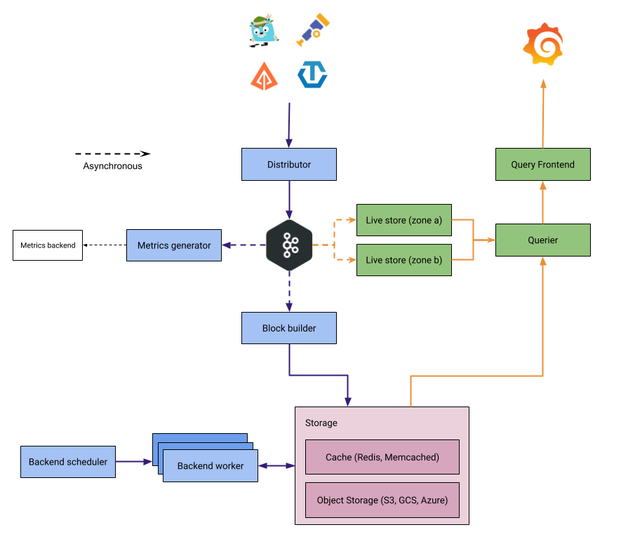
Components
Tempo is made up of the following components.
Distributor
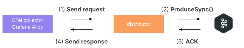
The distributor accepts spans in multiple formats including Jaeger, OpenTelemetry, Zipkin. It uses the receiver layer from the OpenTelemetry Collector. For best performance, it’s recommended to ingest OpenTelemetry Proto. For this reason, Grafana Alloy uses the OTLP exporter/receiver to send spans to Tempo.
Once data is received, the distributor validates the request against limits, shards traces by hashing the traceID, and writes records to Kafka.
The distributor uses the partition ring to determine which partitions are active and routes data accordingly.
A write is only acknowledged to the client after Kafka has confirmed receipt of the data.
Kafka-compatible system
Tempo uses a Kafka-compatible system (such as Apache Kafka or WarpStream) as a durable queue between distributors and downstream components. This serves as a write-ahead log (WAL) that enables the decoupling of write and read paths.
When distributors receive trace data, they shard traces by trace ID and write records to Kafka partitions. Once Kafka acknowledges the write, the distributor returns a response to the client. From this point, the write and read paths diverge:
- Block-builders consume from Kafka to build blocks for long-term object storage.
- Live-stores consume from Kafka to serve recent data queries.
Because traces are sharded by trace ID to specific partitions, both block-builders and live-stores consume unique data without requiring deduplication. This enables Tempo to operate with a replication factor of 1 (RF1) while maintaining durability through Kafka.
Block-builder
The Block-builder is responsible for building blocks which are sent to long-term storage. It does so by consuming from one or more Kafka partitions where distributors have sent trace spans to. The Block-builder organizes spans into blocks based on a configurable time window, for example, 5 minutes.
Live-store
The live-store is a read-path component responsible for serving recent trace data. It consumes trace data from Kafka and makes it available for queries, typically covering the last 30 minutes to 1 hour of data depending on configuration.
Live-stores own the partition lifecycle within Tempo. While Kafka has its own concept of partitions, Tempo maintains a separate partition ring that tracks which Tempo partitions are active and which live-stores own them. Tempo partitions map to Kafka partitions, but they are logically distinct. The partition ring lets Tempo control partition states and ownership independently of Kafka’s internal partition management.
Partitions have three states:
- Pending: No writes or reads. This is the initial state when a new partition is created, waiting for live-stores to be added as owners.
- Active: Normal read-write mode. Distributors send data to active partitions, and queriers read from them.
- Inactive: Read-only mode. Inactive partitions are eventually deleted after a configured period of time.
When a live-store starts, it checks if its partition already exists. If it does, the live-store joins as an owner. If not, it creates a new partition in pending state, waits for memberlist to propagate, then switches it to active. Scaling down requires first marking the partition as inactive while the live-store is still running. After enough time has passed for data to be available in object storage, the partition and live-store can be removed.
For high availability, live-stores are typically deployed across multiple availability zones. Each Tempo partition is owned by one live-store per zone, so if a live-store in one zone becomes unavailable, the live-store in the other zone can continue serving queries. While this setup replicates data across zones (RF2), the read quorum is 1—queriers only need a response from one live-store per partition. This provides high availability without requiring data deduplication on the read path.
Query Frontend
The Query Frontend is the component called by, for example, Grafana when a user wishes to retrieve a specific trace via a trace ID, or carry out a search via a TraceQL filter (for example, all incoming requests for traces). The Query Frontend is responsible for calling one or more Queriers to carry out examination of potential blocks of data where span data for matching traces may exist in parallel, to speed up result response time (dependent on multiple Queriers being configured). Requests by the Query Frontend can be split across multiple Queriers, which all work in parallel to retrieve results quickly. The more Queriers available, generally the quicker a result response. When Queriers have returned enough responses, the Query Frontend is responsible for concatenating all of the span data returned by each individual Querier together to send a response to the requester.
The Query Frontend is responsible for sharding the search space for an incoming query.
A simple HTTP endpoint exposes traces:
GET /api/traces/<traceID>
Internally, the Query Frontend splits the blockID space into a configurable number of shards and queues these requests. Queriers connect to the Query Frontend via a streaming gRPC connection to process these sharded queries.
Querier
Queriers carry out the actual examination of block data in object storage to find any relevant span data based on the trace ID or TraceQL query given. As well as object storage, they also query live-stores for any recent span data that may have been processed but not yet sent to object storage. This ensures that both historical and recent trace data is always available.
The querier finds the requested trace ID in either the live-stores or the backend storage. Depending on parameters, the querier queries the live-stores for recently ingested traces and pulls the bloom filters and indexes from the backend storage to efficiently locate the traces within object storage blocks.
The querier exposes an HTTP endpoint at:
GET /querier/api/traces/<traceID>, but it’s not intended for direct use.
Queries should be sent to the Query Frontend.
Compactor
The compactor is responsible for ensuring that the stored data is both compressed and deduplicated (more on deduplication in the advanced course). The compactor is also responsible for expiring data after the retention period for that data has been reached. Compactors run on scheduled frequent intervals to deal with data that is not compacted and has been stored by the block-builders. Compaction takes into account the data stored for specific traces to minimize search space on queries.
Backend scheduler and worker
The scheduler is a forward-looking re-architecture of the compaction process, with the goal of improving the determinism and removing the duplication present in the current compaction process. The scheduler is responsible for the scheduling and tracking jobs which are assigned to workers for processing. The scheduler component, in combination with the worker, will eventually replace the current compactor component.
The worker connects to the scheduler via gRPC to receive jobs for processing. Workers are responsible for executing jobs assigned to them by the scheduler and updating the job status back to the scheduler. These jobs currently include compaction and retention, but will likely include other kinds of jobs in the future.
The workers currently have the additional responsibility of maintaining the blocklist for all tenants, which was previously handled by the compactor. The determination of which tenants to poll is coordinated through the ring, just as it is with the compactor.
When transitioning from the compactor to the scheduler and worker architecture, some considerations need to be kept in mind:
- Only one scheduler should be running at a time.
- Workers should be scaled up at the same time the compactor is scaled to 0. This is to avoid conflicts between the two systems attempting to compact the same blocks.
Since the worker is taking the role of the compactor when it comes to polling, some documentation may reference the compactor, and can instead be interpreted as the worker for environments where the worker has replaced the compactor.
Object storage
Tempo uses object storage for storing all tracing data. It supports three major object storage APIs:
- Amazon Simple Storage Service (S3)
- Google Cloud Storage (GCS)
- Microsoft Azure Storage (AS)
Metrics-generator
This is an optional component that derives metrics from ingested traces and writes them to a metrics storage. Like live-stores, metrics-generators consume trace data from Kafka. Refer to the metrics-generator documentation to learn more.
Lifecycle of a write
- Trace data is sent from the tracing pipeline (OpenTelemetry Collector, Grafana Alloy) to a distributor.
- The distributor validates the request, shards traces by trace ID, and writes to Kafka.
- Kafka acknowledges the write
- And the distributor returns a response to the client.
- Live-stores consume from Kafka and make data available for recent queries.
- Block-builders consume from Kafka and build blocks for long-term object storage.
Lifecycle of a read
- The query frontend receives a TraceQL query and shards it into jobs for recent data and long-term storage.
- Queriers retrieve recent data from live-stores.
- For older data, queriers fetch blocks from object storage.
- Results are aggregated and returned to the user.
Things to keep in mind
There are three fundamentally important things to keep in mind with traces:
There is no concept of the ’end’ of a trace. A trace can start with any span which holds a unique trace ID that hasn’t been seen by Tempo previously. However, spans can be continually added at any point in the future.
When a trace ID is queried in Tempo, it returns all of the currently stored/ingested spans that belong to that trace and present them in a mapped response (that is, a graph of parent/child/sibling relationships between spans) that allow, for example, Grafana to then visually render those traces.
TraceQL queries return all matching traces from Tempo for the filters presented to it. This does not necessarily mean in chronological order, as some Queriers may return results more promptly than others. When the max trace limit for a TraceQL query has been hit, the Query Frontend will return a response with all the current traces and their spans at that point and ignore/cancel all outstanding Queriers.