Important: This documentation is about an older version. It's relevant only to the release noted, many of the features and functions have been updated or replaced. Please view the current version.
Introduction to time series
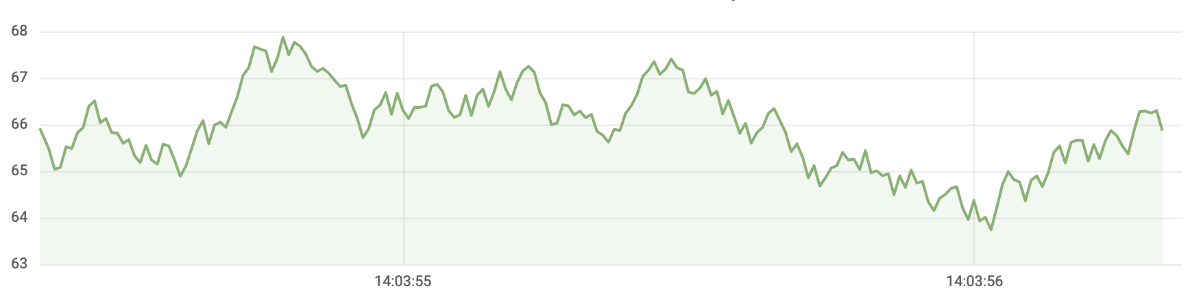
Imagine you wanted to know how the temperature outside changes throughout the day. Once every hour, you’d check the thermometer and write down the time along with the current temperature. After a while, you’d have something like this:
Temperature data like this is one example of what we call a time series—a sequence of measurements, ordered in time. Every row in the table represents one individual measurement at a specific time.
Tables are useful when you want to identify individual measurements but make it difficult to see the big picture. A more common visualization for time series is the graph, which instead places each measurement along a time axis. Visual representations like the graph make it easier to discover patterns and features of the data that otherwise would be difficult to see.
Temperature data like the one in the example, is far from the only example of a time series. Other examples of time series are:
- CPU and memory usage
- Sensor data
- Stock market index
While each of these examples are sequences of chronologically ordered measurements, they also share other attributes:
- New data is appended at the end, at regular intervals—for example, hourly at 09:00, 10:00, 11:00, and so on.
- Measurements are seldom updated after they were added—for example, yesterday’s temperature doesn’t change.
Time series are powerful. They help you understand the past by letting you analyze the state of the system at any point in time. Time series could tell you that the server crashed moments after the free disk space went down to zero.
Time series can also help you predict the future, by uncovering trends in your data. If the number of registered users has been increasing monthly by 4% for the past few months, you can predict how big your user base is going to be at the end of the year.
Some time series have patterns that repeat themselves over a known period. For example, the temperature is typically higher during the day, before it dips down at night. By identifying these periodic, or seasonal, time series, you can make confident predictions about the next period. If we know that the system load peaks every day around 18:00, we can add more machines right before.
Aggregating time series
Depending on what you’re measuring, the data can vary greatly. What if you wanted to compare periods longer than the interval between measurements? If you’d measure the temperature once every hour, you’d end up with 24 data points per day. To compare the temperature in August over the years, you’d have to combine the 31 times 24 data points into one.
Combining a collection of measurements is called aggregation. There are several ways to aggregate time series data. Here are some common ones:
- Average returns the sum of all values divided by the total number of values.
- Min and Max return the smallest, and largest value in the collection.
- Sum returns the sum of all values in the collection.
- Count returns the number of values in the collection.
For example, by aggregating the data in a month, you can determine that August 2017 was, on average, warmer than the year before. Instead, to see which month had the highest temperature, you’d compare the maximum temperature for each month.
How you choose to aggregate your time series data is an important decision and depends on the story you want to tell with your data. It’s common to use different aggregations to visualize the same time series data in different ways.
Time series and monitoring
In the IT industry, time series data is often collected to monitor things like infrastructure, hardware, or application events. Machine-generated time series data is typically collected with short intervals, which allows you to react to any unexpected changes, moments after they occur. As a consequence, data accumulates at a rapid pace, making it vital to have a way to store and query data efficiently. As a result, databases optimized for time series data have seen a rise in popularity in recent years.
Time series databases
A time series database (TSDB) is a database explicitly designed for time series data. While it’s possible to use any regular database to store measurements, a TSDB comes with some useful optimizations.
Modern time series databases take advantage of the fact that measurements are only ever appended, and rarely updated or removed. For example, the timestamps for each measurement change very little over time, which results in redundant data being stored.
Look at this sequence of Unix timestamps:
1572524345, 1572524375, 1572524404, 1572524434, 1572524464Looking at these timestamps, they all start with 1572524, leading to poor use of disk space. Instead, we could store each subsequent timestamp as the difference, or delta, from the first one:
1572524345, +30, +29, +30, +30We could even take it a step further, by calculating the deltas of these deltas:
1572524345, +30, -1, +1, +0If measurements are taken at regular intervals, most of these delta-of-deltas will be 0. Because of optimizations like these, TSDBs uses drastically less space than other databases.
Another feature of a TSDB is the ability to filter measurements using tags. Each data point is labeled with a tag that adds context information, such as where the measurement was taken. Here’s an example of the InfluxDB data format that demonstrates how each measurement is stored.
Here are some of the TSDBs supported by Grafana:
weather,location=us-midwest temperature=82 1465839830100400200
  |    -------------------- --------------  |
  |             |             |             |
  |             |             |             |
+-----------+--------+-+---------+-+---------+
|measurement|,tag_set| |field_set| |timestamp|
+-----------+--------+-+---------+-+---------+
Collecting time series data
Now that we have a place to store our time series, how do we actually gather the measurements? To collect time series data, you’d typically install a collector on the device, machine, or instance you want to monitor. Some collectors are made with a specific database in mind, and some support different output destinations.
Here are some examples of collectors:
A collector either pushes data to a database or lets the database pull the data from it. Both methods come with their own set of pros and cons:
Since it would be inefficient to write every measurement to the database, collectors pre-aggregate the data and write to the time series database at regular intervals.