Documentation Grafana Cloud Observe and act Instrument and send data Traces Introduction Tempo architecture

Tempo architecture

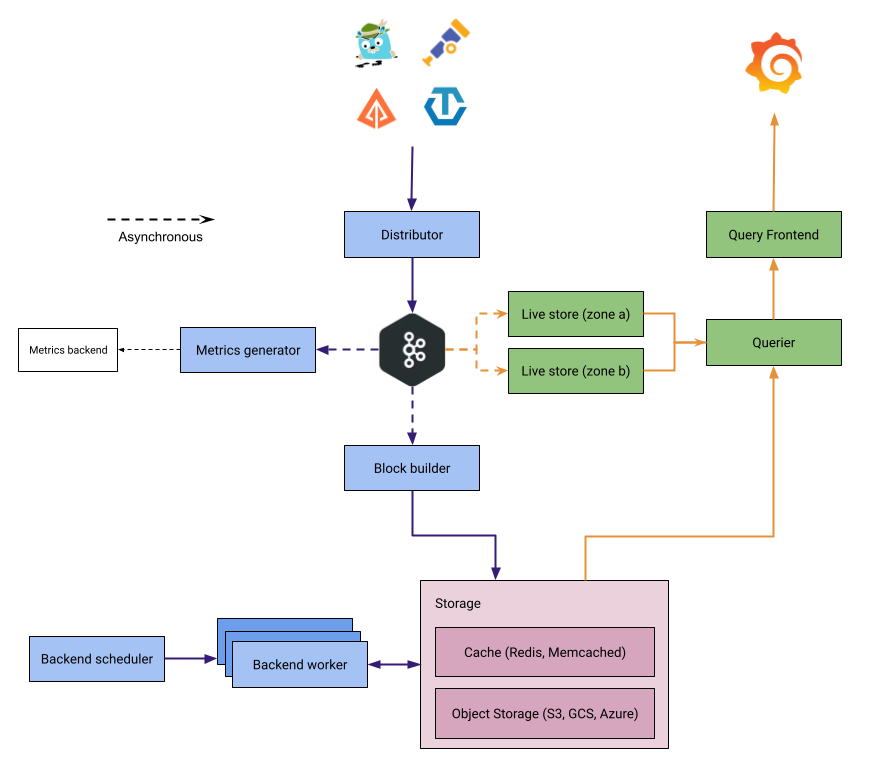
The journey of a trace is usually from an instrumented application, to a trace receiver/collector, to a trace backend store, and then those traces are retrieved and visualized in a tool like Grafana.

Grafana Tempo acts in two major capacities:

• Ingesting trace spans, sorting the span resources and attributes into columns in an Apache Parquet schema, before sending them to object storage for long-term retention.
• Retrieving trace data from storage, either by specific trace ID or by search parameters using TraceQL.

This page gives a high-level overview of how Tempo works: how it ingests, stores, and queries trace data, and the components that make up a Tempo deployment. For in-depth operational detail, refer to the Tempo architecture reference.

Design goals

The Tempo architecture is built around a few goals that shape how it ingests, stores, and queries traces.

• Cost-efficient storage: Tempo stores all trace data in object storage.
• Independent scaling: In microservices mode, Tempo separates the write path from the read path, so you can scale ingestion and query capacity independently.
• Durability without extra replication: In microservices mode, a Kafka-compatible queue acts as a write-ahead log (WAL). After Kafka acknowledges a write, the data is durable, so Tempo doesn’t replicate data across instances on the write path and can operate with a replication factor of 1 (RF1), which reduces cost.
• Efficient attribute queries: Tempo stores blocks in Apache Parquet, a columnar format, so a query reads only the columns it needs instead of scanning entire traces.

Deployment modes

All Tempo components are compiled into the same binary; the -target parameter controls which components run in a given process, whether that’s one process running everything or many processes each running one component. This lets you run Tempo in two modes:

• Monolithic mode: All required components run in a single process (-target=all, the default). No Kafka is required; the distributor pushes trace data in-process to the live-store and metrics-generator.
• Microservices mode: Each component runs as a separate process with its own -target. This mode requires a Kafka-compatible system and is recommended for production.

Object storage is recommended for production in both modes; a local filesystem backend is available for development and testing.

For more information, refer to Deployment modes and Set up for tracing.

How data flows

Tempo separates the write path, which gets trace data into storage, from the read path, which serves queries.

Lifecycle of a write

The following steps describe the write path in microservices mode. In monolithic mode, the distributor pushes data in-process to the live-store and metrics-generator instead of writing to Kafka.

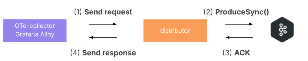
1. Trace data is sent from the tracing pipeline (OpenTelemetry Collector, Grafana Alloy) to a distributor.

2. The distributor validates the request, shards traces by trace ID, and writes to Kafka.

3. Kafka acknowledges the write, and the distributor returns a response to the client.

   After the write is acknowledged, downstream components consume the data asynchronously:

4. Live-stores consume from Kafka and make data available for recent queries.

5. Block-builders consume from Kafka and build blocks for long-term object storage.

6. Metrics-generators (optional) consume from Kafka to derive metrics from traces.

Lifecycle of a read

1. The query frontend receives a query and shards it into jobs for recent data and long-term storage.
2. Queriers retrieve recent data from live-stores.
3. For older data, queriers fetch blocks from object storage.
4. Results are aggregated and returned to the user.

Components

The following table summarizes the Tempo components and which deployment modes use them.

Storage

Tempo stores all trace data in object storage. It supports three major object storage APIs:

• Amazon S3 (and S3-compatible systems, such as MinIO)
• Google Cloud Storage (GCS)
• Microsoft Azure Blob Storage

A local filesystem backend is available for development and testing.

Trace data is stored in Apache Parquet blocks, a columnar format that lets queries read only the attributes they need. Backend workers enforce retention by expiring data in object storage after the configured retention period.

For more information, refer to Object storage and Block format.

What you can query

Tempo answers two kinds of read requests: lookups for a specific trace by trace ID, and searches across traces using TraceQL, the Tempo trace query language. You can also compute TraceQL metrics (for example, span rates and latency quantiles) directly from trace data, and use the optional metrics-generator to produce rate, error, and duration (RED) metrics and service graphs.

Tempo ingests traces in OpenTelemetry (OTLP), Jaeger, and Zipkin formats.

Tempo is multi-tenant: trace data is isolated per tenant at the storage level. For more information, refer to multi-tenancy.

For the span fields and attributes you can query, refer to Trace structure. For AI-driven access to trace data through the MCP server and LLM-optimized APIs, refer to Tempo and AI.

Component details

The following sections describe each component in a little more detail. For full operational reference, follow the link at the end of each section.

Distributor

The distributor is the entry point for trace data. It accepts spans in OTLP (recommended), Jaeger, and Zipkin formats and validates them against per-tenant ingestion limits. In microservices mode, it shards traces by trace ID and writes them to Kafka; in monolithic mode, it pushes data in-process to the live-store and metrics-generator.

For more information, refer to Distributor.

Kafka-compatible queue

In microservices mode, Tempo uses a Kafka-compatible system (such as Apache Kafka or WarpStream) as a durable write-ahead log between the distributor and downstream consumers. Because Kafka provides durability after it acknowledges a write, Tempo can operate at a replication factor of 1. Kafka isn’t used in monolithic mode.

For more information, refer to Kafka.

Block-builder

The block-builder consumes trace data from Kafka, organizes spans into Apache Parquet blocks, and flushes them to object storage for long-term retention. It runs only in microservices mode; in monolithic mode, the live-store flushes blocks to object storage directly. For details, refer to Block-builder.

Live-store

The live-store serves recent trace data, holding traces in memory and in a local write-ahead log so they’re queryable within seconds of ingestion. In microservices mode, it consumes trace data from Kafka; in monolithic mode, it receives data directly from the distributor. For high availability, live-stores can be deployed across availability zones.

For more information, refer to Live-store.

Query frontend

The query frontend is the entry point for queries. It receives TraceQL queries and trace ID lookups, shards each into parallel jobs that it distributes to queriers, and merges the returned results into a final response.

For more information, refer to Query frontend.

Querier

The querier executes the jobs dispatched by the query frontend. It fetches recent data from live-stores and historical data from object storage, then returns results to the query frontend for merging.

For more information, refer to Querier.

Backend scheduler and worker

The backend scheduler and worker handle compaction, retention, and blocklist maintenance for data in object storage. The scheduler creates jobs and assigns them to workers, which compact small blocks into larger ones and expire data past its retention period. Together they replace the legacy compactor.

For more information, refer to Compaction.

Metrics-generator

The metrics-generator is an optional component that derives rate, error, and duration metrics and service graphs from traces and remote-writes them to a metrics backend such as Prometheus or Grafana Mimir.

For more information, refer to Metrics-generator.

Object storage

Object storage is the long-term store for all trace data. Tempo supports Amazon S3 (and S3-compatible systems), Google Cloud Storage, and Azure Blob Storage, with a local filesystem backend for development and testing.

For more information, refer to Object storage.

Things to keep in mind

There are three fundamentally important things to keep in mind with traces:

• There’s no concept of the ’end’ of a trace. A trace can start with any span which holds a unique trace ID that hasn’t been seen by Tempo previously. However, spans can be continually added at any point in the future.
• When a trace ID is queried in Tempo, it returns all of the currently stored/ingested spans that belong to that trace and presents them in a mapped response (that is, a graph of parent/child/sibling relationships between spans) that allows, for example, Grafana to then visually render those traces.
• TraceQL queries return all matching traces from Tempo for the filters presented to it. This doesn’t necessarily mean in chronological order, as some queriers may return results more promptly than others. When the maximum trace limit for a TraceQL query has been hit, the query frontend returns a response with the traces and spans it has collected so far and stops waiting for outstanding queriers.

Next steps

• Plan and deploy Tempo: Set up for tracing.
• Explore the architecture in depth: Tempo architecture reference.
• Learn the parts of a span: Trace structure.