Documentation Grafana Enterprise Metrics documentation Graphite proxy Graphite querier

Graphite querier

The Graphite querier provides the Graphite querying API, for more information about the API refer to the Graphite documentation.

Supported Graphite functions

The Graphite querier comes with a set of built-in functions which tend to execute faster than the original Graphite implementation, we refer to these built-in functions as the “native query engine”. The native query engine only implements a set of very commonly used functions, many of the less commonly used functions are missing from it. Whenever the Graphite querier receives a query which includes a function that it doesn’t have in the native query engine it offloads the function processing to a stock Graphite deployment (if available). To learn more about how the Graphite querier offloads the function processing to a separate Graphite process, refer to Offloading the function processing to Graphite.

The native query engine is imported from an open source project called CarbonAPI, for more information about its function library and which functions are/aren’t implemented, refer to the CarbonAPI repository.

Query handling

The query handling endpoint accepts Graphite queries, it processes them in the following steps. This is a simplification which ignores the fact that some steps in the process are cached.

Parsing the query

The query gets parsed and based on the used functions a decision is made which query engine shall be used. Whenever all used functions are supported by the native query engine then this one is used, otherwise the Graphite function processing will be off-loaded to the external Graphite process.

The metric name patterns get extracted from the query and a Prometheus query gets generated to fetch the required data to serve the query from Grafana Mimir. To generate that Prometheus query the name mapping schemes get applied in reverse, for more information about the name mapping schema refer to Graphite write proxy.

Breaking the query up into sub-queries

If the original query is requesting a long time range, then it gets broken up into sub-queries. Each sub-query has a maximum time range of 1d by default, configurable via the flag graphite.querier.split-queries-by-interval, the time range boundaries are aligned to multiples of the split interval. The default sub-query length of 1d is derived from the fact that by default the blocks in the store have a length of 1d after compaction, that way each sub-query processes exactly one block.

Each sub-query gets assigned two points budgets defining how many data points it may produce, the two budgets are called soft budget and hard budget. The points budgets per sub-query get calculated based on the total query budgets configured via the flags graphite.querier.max-points-per-req-{soft,hard} which by default have the values 1000000 and 20000000, each sub-query gets an equal share which is proportionate to the total queried time range.

The soft budget defines to what number of points the results should optimally be aggregated, but it may be exceeded if it is not possible to stay within the soft budget due to the configured retentions in the storage-schemas. If the number of points can’t be reduced to fit within the hard budget then the query directly errors to prevent overloading of the query engine.

Note that the sub-queries are only responsible for fetching and processing the raw data in preparation for the query engine to run on top of the data. The query engine will later run on the combined sub-query results and not on each sub-query result separately.

Processing of the sub-queries

The sub-queries which resulted from breaking up the original query get processed concurrently by a pool of worker threads. The size of the work pool is configurable via the flag graphite.querier.query-handling-concurrency, with a default value of 8. Increasing the worker pool size can speed up the processing of queries with long time ranges because they will be processed at a higher concurrency as long as enough physical cores are available, but it will also increase the memory consumption.

Fetching the data

Each sub-query worker separately fetches the data which it requires to process its sub-query from Grafana Mimir. This means that if one Graphite query gets broken up into 5 sub-queries then Grafana Mimir sees 5 separate queries, so it is expected that the Grafana Mimir query rate might be higher than the Graphite query rate.

Choosing the target interval for each metric

Each metric will get aligned to an interval that is determined based on the tenant’s storage-schemas configuration. First the metrics get grouped by the schemas of which they match the pattern, these groups are called rollup groups because they always get rolled up (horizontally aggregated) together, then each rollup group’s target interval gets determined based on the queried time range and the schema configuration. For this the time range of the original Graphite query is used and not the time range of the sub-query. To learn more details about the process of determining the target interval, refer to Storage schemas.

After each rollup group has an assigned target interval the total number of points which this sub-query is going to generate gets calculated based on the number of metrics in each rollup group, their assigned target intervals, and the time range of the sub-query.

If the total number of points which will get generated by this sub-query exceeds the sub-query’s soft budget then the rollup group which currently has the lowest target interval gets bumped to the next retention of its matching storage schema. Since the retentions are always defined in increasing interval order, bumping a rollup group to the next retention results in less points being generated. This process gets repeated until either the total number of points generated by the sub-query fits in the soft budget or all rollup groups have already been bumped to their final retention.

If the total number of points which will get generated by this sub-query still exceeds the sub-query’s hard budget then an error gets returned and the query processing gets aborted.

Alignment and aggregation of the data

The data points of each metric now get aligned to the target interval of the rollup group which the metric is in. If there are data points with time stamps that are not a multiple of the target interval then they get aligned to multiples of the interval by shifting them to a lower time stamp. If there are multiple data points within one interval then they get aggregated together by the aggregation function chosen based on the storage-aggregation’s configuration of the tenant, the resulting value will be assigned with a timestamp that is a multiple of the target interval. To learn more about the storage-aggregation refer to Storage aggregations.

This process is cached, but the caching logic is omitted in this description for the sake of simplicity, to learn more about the caching logic refer to Caching.

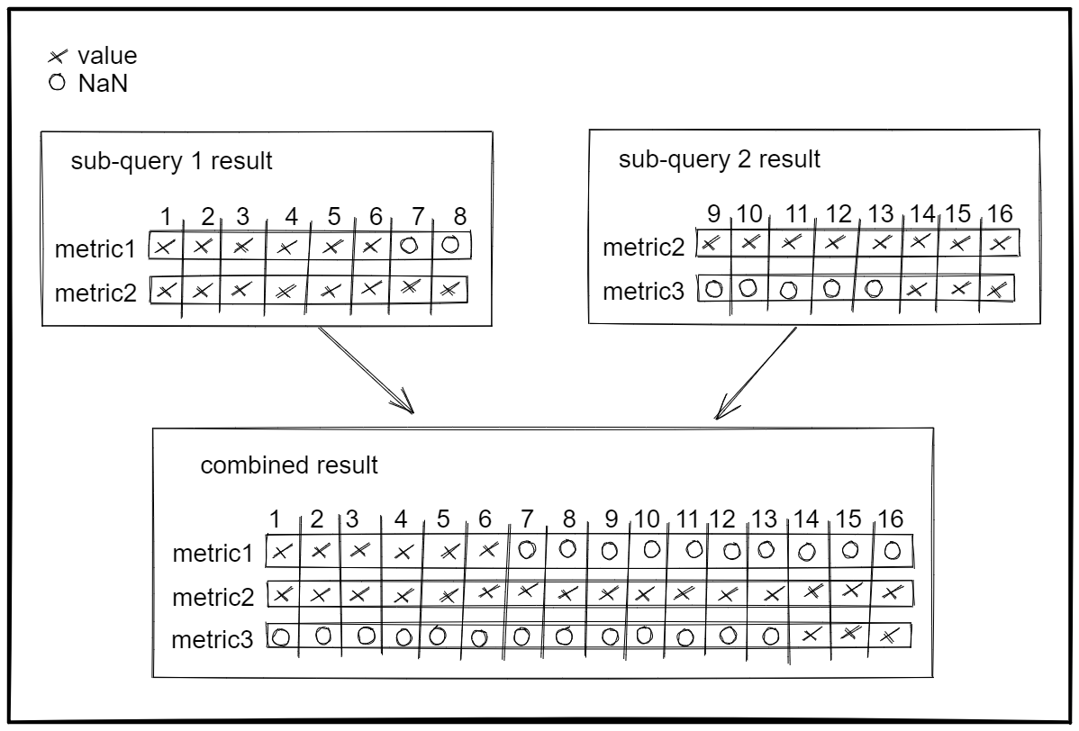
Combining the sub-query results

Each sub-query returns a set of metrics that has been aligned and aggregated to the correct interval, now the results of the different sub-queries get combined into one set of metrics.

If a sub-query result contains a metric which is not present in another sub-query result then the gap is filled with NaN.

At this point it is possible that the same metric has been aggregated to different intervals in the different sub-queries, because if one sub-query resulted in a larger number of metrics than another then its retention might have been bumped to fit the number of points generated by the sub-query into its soft budget In this situation the sub-query results with the lower interval get aggregated to match the interval of the sub-query result with the higher interval, because the Graphite query engines require each metric to have a constant interval.

The result after combining the sub-query results is one set of metrics, where each metric is guaranteed to have a consistent interval and each metric has data points filling the entire queried time range because all gaps have been filled with NaN values.

Function processing

The combined sub-query results now get passed into the query engine that has been chosen in the beginning of the query handling process. This can either be the native query engine (preferred) or a an optional Graphite deployment running in a separate process (for function completeness). To learn more about how the Graphite querier offloads the function processing to a separate Graphite process, refer to Offloading the function processing to Graphite.

Returning to the user

The query engine returns a set of metrics which has been generated by running the Graphite functions specified in the query on the combined sub-query results, this set of metrics now gets returned to the user.

Illustration

This is an illustration of the above described query handling process:

Caching

The aggregation work which is performed as part of the query handling gets cached in order to minimize the latency of queries that request the same metrics with overlapping time ranges multiple times. The caching happens in chunks of data, where each chunk has a size of 1d by default, configurable via -graphite.querier.split-queries-by-interval. The boundaries of the cached chunks are always multiples of the chunk size in UTC, meaning that each chunk contains the data of one day from midnight to midnight in UTC by default. Partial chunks don’t get cached, they get regenerated at every query.

Imagine a Grafana dashboard querying a given set of metrics with a constant time range length of 3d applied relative to the current time.

• The first query requests the time range 2021-01-10T13:25:00Z - 2021-01-12T13:25:00Z
  • The sub-query result for the time range 2021-01-10T13:25:00Z - 2021-01-11T00:00:00Z gets generated but it can’t be cached because it is partial
  • The sub-query result for the time range 2021-01-11T00:00:00Z - 2021-01-12T00:00:00Z gets generated and cached
  • The sub-query result for the time range 2021-01-12T00:00:00Z - 2021-01-12T13:25:00Z gets generated but it can’t be cached because it is partial
• The Grafana dashboard refreshes again 1min later
• Now the new query is requesting the time range 2021-01-10T13:26:00Z - 2021-01-12T13:26:00Z
  • The sub-query result for the time range 2021-01-10T13:26:00Z - 2021-01-11T00:00:00Z gets generated but it can’t be cached because it is partial
  • The sub-query result for the time range 2021-01-11T00:00:00Z - 2021-01-12T00:00:00Z gets retrieved from the cache
  • The sub-query result for the time range 2021-01-12T00:00:00Z - 2021-01-12T13:26:00Z gets generated but it can’t be cached because it is partial

This means the data fetching, the alignment and the aggregation of the data of the entire day 2021-01-11 is omitted. The caching is especially effective for queries that query for long time ranges. There are two caches involved in this, they are named metric name cache and aggregation cache.

Metric name cache

The metric name cache caches the resolution of metric name patterns that are used in the queries into lists of concrete metric names. Each entry in the metric name cache contains a list of metric names corresponding to a combination of the following attributes:

• Metric name pattern
• Time range

Aggregation cache

The aggregation cache caches the aligned and aggregated results of sub-queries on a per-metrics basis. Each entry in the aggregation cache contains a chunk of data corresponding to a combination of the following attributes:

• Metric name
• Time range with a length of 1d by default
• Target interval
• Aggregation function used

Cache usage

This illustrates the flow how these two caches are used in the query handling process.

Offloading the function processing to Graphite

The Graphite querier’s native query engine only implements an incomplete set of Graphite functions, whenever a query involves a Graphite function that is not implemented in the native query engine then the Graphite querier offloads the function processing to a Graphite deployment which runs in a separate process.

It does this by forwarding the original query to the Graphite process, just like a simple reverse HTTP Proxy. The Graphite process is configured to use the Graphite querier as a cluster server, because it doesn’t have the necessary data to serve the query locally it will then reach out to the Graphite querier to fetch the raw data via a separate call to the /graphite/render endpoint which queries only for the data without any Graphite functions in the query.

The Graphite querier will then handle this second query which it received just like any other query and it will return the queried data to the client, which in this case is the Graphite process. In the process of handling this query the Graphite querier will still perform all the necessary aggregations on the queried data and aggregate it based on the configured storage-schemas, storage-aggregations and the max-points-per-req-soft parameter.

The Graphite process then executes the functions specified in the query on the data it received from the Graphite querier and returns the result back to the Graphite querier by replying to the original request that the Graphite querier has forwarded to it.

The Graphite querier then proxies the response from the Graphite process back to the user.

We recommend using this image to deploy the Graphite process, because it allows the configuration of the CLUSTER_SERVERS via the env var GRAPHITE_CLUSTER_SERVERS:

Copy

docker.io/raintank/graphite-mt:8-7ebde4c60

A valid configuration example via the environment variables in a Kubernetes deployment looks like this, this assumes that the Graphite querier is reachable on the address graphite-querier on port 80:

Copy

        - name: GRAPHITE_CLUSTER_SERVERS
          value: graphite-querier:80/graphite

The chain of calls looks like this, where the graphite-querier might or might not be the same process:

Copy

client -> graphite-querier -> graphite -> graphite-querier -> GEM Querier

Querying the remote read API

For enhanced internal query performance, the Graphite querier performs the queries against the Prometheus remote read API. The only configuration required is the query address, as described in this configuration example:

yaml Copy

    -graphite.querier.query-address: 'http://<current server-http-listen-address>:<current server-http-listen-port>',

Regarding graphite.querier.query-address we should make some clarifications:

• The address should point to the Grafana Mimir query frontend to benefit from its capabilities.
• If the Query Frontend or Grafana Mimir is configured with an http prefix, then you need to add it at the end of the query address to make it consistent. Otherwise, graphite won’t be able to query the right querier address.
• If you are running the single binary installation then this address will be localhost and unless you have a specific http prefix then you can skip the -graphite.querier.query-address flag entirely.