Grafana Loki query acceleration: How we sped up queries without adding resources

As we discussed when we rolled out the latest major release of Grafana Loki, we’ve grown the log aggregation system over the past five years by balancing feature development with supporting users at scale. A big part of the latter has been making queries much faster — and that was a major focus with Loki 3.0 too. 

We’ve seen peak query throughput grow from 10 GB/s in our Loki 1.0 days to greater than 1 TB/s even before 3.0. However, to grow further, and to make sure we are staying true to our principles of being cost effective and easy to use for developers, we are always looking for opportunities to be smarter.

For example, we recently noticed a funny thing with filter queries: They touch a lot of data they don’t need to. Over a seven-day period, our Grafana Labs prod clusters processed 280 PB of logs. From that total, about 140 PB of the searched logs didn’t match any of the filtering expressions. In other words, 50% of the searched data returned no results! To make things worse, 65% of the processed data (182 PBs) only returned up to one log line for every 1 million logs. 

Of course, we could have solved the throughput problems by throwing more compute resources at it, but that doesn’t align with our vision of making Loki cost-effective and scalable. Instead, we saw this as a challenge and an opportunity. How could we improve the experience of these faster-returning filter queries, while still maintaining Loki’s ease of use and cost effectiveness principles? 

Enter query acceleration, an experimental feature included in Loki 3.0.

How we approached query acceleration in Loki

Before diving in, we should quickly cover two concepts we’ll use in this blog post: n-grams and Bloom filters.

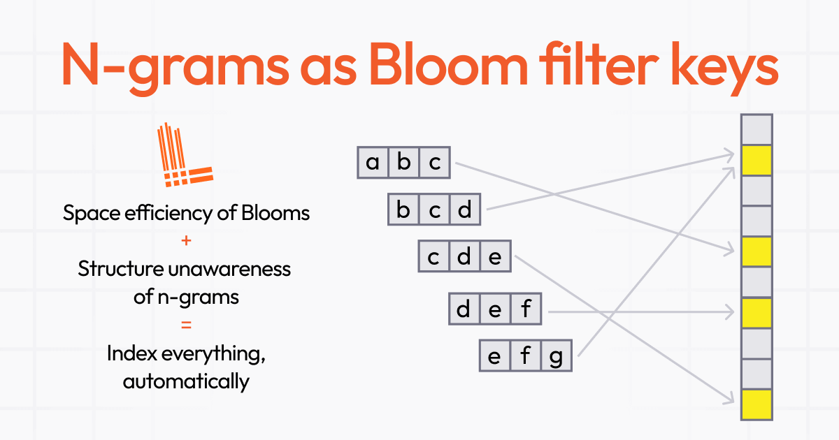
• We use n-grams as permutations of substrings. For example, given the string “abcdef,” the different trigrams (n-grams where n=3) are “abc,” “bcd,” “cde,” and “def.”
• Bloom filters are data structures that allow for probabilistic matching. They allow for some false positives, but not for false negatives. They have a long history of usage in the database space.

As mentioned above, we observed that most data was irrelevant at query time — it never had a chance of being valuable for that particular query. So we realized that identifying and eliminating that irrelevant data was essentially the same as only searching for relevant data. Furthermore, because we chose to focus on “where the data isn’t,” we looked for a space-effective data structure that provided us with a “good enough” estimate of where the relevant data for a filter query might be, which would then allow us to disregard the rest of the data.

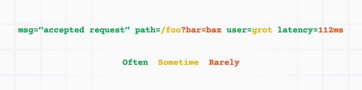
The other key ingredient was n-grams. They allowed us to maintain the “structure unawareness” that makes Loki so easy to use (no schemas). It created a lot of data, but we benefited from the fact that many log lines have common information. For example, all the text highlighted in green below showcase repeated text throughout different logs — the so-called common information.

msg=”adding item to cart” userID=”a4hbfer74g” itemID=”jr8fdnasd65u4”

msg=”adding item to cart” userID=”a4hbfer74g” itemID=”78kjasdj4hs21”

msg=”adding item to cart” userID=”h74jndvys6” itemID=”yclk37uzs95j8”

Luckily, the nature of Bloom filters means duplicates are free, so the entropy of log lines helped us tackle the space (cost) problem.

Adding it all up, we ended up with the following approach, which we’ll dig into more in the next section:

This means that all filter queries can conceivably benefit from Blooms, which, by the way, we’re currently seeing are about 2% of the size of the logs themselves.

On top of everything we’ve already discussed, query acceleration also ships with a brand new query sharding strategy where we leverage Bloom filters to come up with fewer and fairer query shards. 

Traditionally, by analyzing TSDB index statistics, Loki would determine the nearest power of two for dividing data into shards that are, in theory, of approximately equal size. Unfortunately, this is often not the case when some series have considerably more data than others. As a result, some shards would end up processing more data than others.

We now use Bloom filters to reduce the number of chunks to be processed right away during the planning phase in the query frontend, and to evenly distribute the amount of chunks each sharded query will need to process.

How the Bloom filter components work

Let’s dive a bit into how Bloom filters are created and how they are used for matching filtering expressions. We have introduced two new components: the Bloom compactor and the Bloom gateway.

The Bloom compactor builds Bloom filters from the chunks in the object store. We build one Bloom per series and aggregate them together into block files. Series in Bloom blocks follow the same ordering scheme as Loki’s TSDB and sharding calculation. This gives a data locality benefit when querying, as series in the same shard are likely to be in the same block. In addition to blocks, compactors maintain a list of metadata files containing references to Bloom blocks and the TSDB index files they were built from.

Bloom compactors are horizontally scalable, and they use a ring to shard tenants and claim ownership of subsets of the series key-space. For a given series, the compactor owning that series will iterate through all the log lines inside its chunks and build a Bloom. For each log line, we compute its n-grams and append to the Bloom both the hash for each n-gram and the hash for each n-gram plus the chunk identifier. The former allows gateways to skip whole series, while the latter is for skipping individual chunks.

For example, given a log line “abcdef” in the chunk “aaf67d”, we compute its n-grams: “abc”, “bcd”, “cde”, “def”. And append to the series Bloom hash(“abc”), hash(“abc” + “aaf67d”) … hash(“def”), hash(“def” + ““aaf67d”).

On the other end, Bloom gateways handle chunks filtering requests from the index gateway. The service takes a list of chunks and a filtering expression and matches them against the Bloom filters, removing those chunks not matching the given filter expression.

Like Bloom compactors, the new gateways are also horizontally scalable and use the ring for the same purpose as the compactor: sharding tenants and series key-spaces. Index gateways use the ring to determine which Bloom gateway they should send chunks filtering requests, based on the series fingerprints for those chunks.

By adding n-grams to Bloom filters in the compactors instead of whole log lines, Bloom gateways can perform partial matches. For the example above, a filter expression |= “abcd” would yield two n-grams: “abc” and “bcd”. Both would match against the Bloom.

Now for each chunk within the series, we can test the Bloom again by appending the chunk ID to the n-gram.

Taken collectively, the following diagram showcases how we build blooms and how do we use them to skip series and blocks not matching the n-grams from a filtering expression:

N-grams sizes are configurable. The longer the n-gram, the fewer tokens we need to append to the Bloom filters. However, the longer filtering expressions need to be able to check them against Bloom filters. For the example above, where the n-gram length is 3, we need filtering expressions that have at least 3 characters.

Creating a good user experience

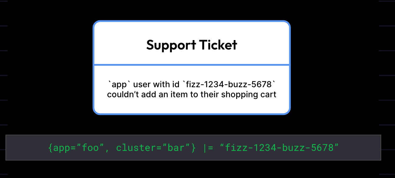
Of course, our primary objective here is making queries return data faster! This approach tends to work even better for specifically small “needles,” such as finding a UUID, or other rarely occurring string.

Bloom filters are particularly useful for precise searches — for instance, if you’re looking for all logs that mention a specific customer ID or a unique error code. We find this is a very common pattern for developers and support engineers who use Loki. Because Bloom filters allow Loki to process just the logs likely to contain those terms, and these terms likely appear in very few log lines, the impact to search times is significant. 

And all signs point to Bloom filters being really effective. Early internal tests suggest that with Bloom filters, Loki can skip a significant percentage of log data while running queries. Our dev environment tests show that we can now filter out between 70% and 90% of the chunks we previously needed to process a query. 

Here is an example of the results we’re seeing when running one of these “needle in a haystack” searches with Bloom filters. This query includes several filtering conditions and represents a typical use case we’ve seen our customers run on Grafana Cloud Logs, which is powered by Loki.

A note of caution on use cases

Not every query will benefit from Bloom filters in our current implementation. Let’s walk through the conditions where Bloom filters would and would not be invoked:

The following condition should be satisfied for a query to use blooms:

• Queries should contain at least one filtering expression. Whereas {env=“prod”} |= “order=17863472” | logfmt  would use Bloom filters,  {env=“prod”} | logmt would not.

However, the following will prevent a query from leveraging blooms:

• Bloom filters are not used for not-equal filters: both regular and regex filters. Neither != “debug” nor !~ “(staging|dev) will use Bloom filters. 
• Filtering expressions after line formatting expressions won’t use Bloom filters. For example |= `level=“error”` | logfmt | line_format “ERROR {{.err}}” |= `traceID=“3ksn8d4jj3”` where |= `level=“error”` will benefit from Bloom filters but |= `traceID=“3ksn8d4jj3”` will not.
• Queries for which Bloom blocks haven’t been downloaded yet on the Bloom gateways.

We were also able to implement this in a way that held true to one of our other Loki ease of use principles: schemaless at scale. Because of this, the query experience looks the exact same, apart from data returning faster. You can still ingest data the same way. And when we unveil this in Grafana Cloud, no configuration will be necessary to use Blooms on the client side.

Looking ahead

This is an extremely promising experimental feature, but this is just the beginning. We’ve made it work: now it’s time to make it simpler and even faster! To learn more about query acceleration, and learning about how to enable it in your Loki cluster, checkout the Loki 3.0 docs.

Grafana Cloud is the easiest way to get started with metrics, logs, traces, dashboards, and more. We have a generous forever-free tier and plans for every use case. Sign up for free now!