How to calculate the difference of a value over time with InfluxDB and Grafana
Learning about the past helps us understand the present, and even predict the future. So, whether you are monitoring CPU usage or how long your IoT device was powered on and then off, at some point, you might want to know the difference of a value over time.
InfluxDB is an open source database for storing and retrieving time series data. Thanks to its own query languages — flux and InfluxQL — it provides different and powerful ways to analyze data. And to make sense of all that data in an intelligible and more intuitive way, you can use Grafana.
In this blog post, we’ll look at how you can use Grafana to visualize data returned from an InfluxDB query that uses the built-in difference() function.
Using Grafana and InfluxDB: A step-by-step example
Note: To follow along with this post — and to visualize InfluxDB data in Grafana — add and configure the InfluxDB data source to your Connections, if you haven’t already.
To get started, let’s consider the below InfluxDB database named “cpu_load.” It has a timestamp (in nanosecond-precision Unix time), a server name (cs30), a tag containing metadata about the server location (emea_west), and, lastly, a value field (e.g., 0.56).
1696321929371835915 cs30 emea_west 0.56
1696322083725184366 cs30 emea_west 0.76
1696322090789971557 cs30 emea_west 0.78
1696322093558034654 cs30 emea_west 0.35
1696322099153723182 cs30 emea_west 0.65
1696406363443417871 cs30 emea_west 0.9
1696406367178746980 cs30 emea_west 0.92
1696406370058539266 cs30 emea_west 0.99
1696406372466320956 cs30 emea_west 0.99
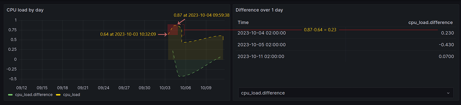
1696406378586702043 cs30 emea_west 0.87As mentioned above, the timestamps in this dataset are in Unix time (seconds since the epoch). The oldest data point, at the top, was written in the database on October 3, 2023 at 8:32:09 GMT. The most recent data point, at the bottom, was written on October 4, 2023 at 7:59:38 GMT.
If we want to know the difference of the CPU load between the most recent data point, which has a value of 0.87, and the oldest data point, which was written one day (1d) prior and has a value of 0.56, we can use the following query:
SELECT difference(last(value)) FROM cpu_load
WHERE time >= now() - 1d
GROUP BY time(1d)
The outcome of this query in this example would look like this:
Time                  cpu.difference
*******************   **************
2023-10-04 02:00:00   0.310
This outcome shows that the difference between the most recent value in our database (0.87) and the point in the past (0.56) — which was captured one day earlier — would be 0.310. This is right, because 0.87-0.56 = 0.31.
One way to understand this query is to think about it like this: You are choosing a point in the past, and, to order the results, you are also choosing a minimum timeframe that must have passed between that measurement in the past and the latest measurement written in the database.
But what exactly happens under the hood? Let’s break down the query.
In our SELECT clause, we are using two functions: difference() and last().
The difference() function returns the difference between two values. The last(value) function specifies that we want to look at the field value with the most recent timestamp. The parameter value in the last(value) function refers to the InfluxDB field that stores the value of a measurement, which in our case is 0.87.
In the WHERE clause, we are specifying how far back from the present day we want to look to compare the last value from our SELECT. In this example, we chose 1 day (1d).
Finally, because the difference() function requires a GROUP BY interval, we set a time interval to order the query results by time, which in turn requires the time() function. The time() function accepts duration data type format (seconds, minutes, hours, days). In this example, we chose a time interval of 1d, so the query results into 1-day groups across the time range specified in the WHERE clause.
To use this InfluxQL query in Grafana:
- Toggle the menu at the top left corner
- Click Explore
- Select InfluxDB from the data source drop-down menu
- Click on the Edit button to switch to raw query mode
- Copy/paste the query in the text area
- Click Run query
- Click Add to dashboard, so you can visualize the data in a panel

Wrapping up and next steps
Grafana’s “big tent” philosophy means you can visualize data from a wide range of data sources — including InfluxDB. For more information on how to use InfluxDB and Grafana, check out our technical documentation, which includes this detailed guide for getting started.
Grafana Cloud is the easiest way to get started with metrics, logs, traces, and dashboards. For a look at our generous forever-free tier and plans for every use case, sign up now!