Less is more: How Grafana Mimir queries run faster and more cost efficiently with fewer indexes
Over the past six months, we have been working on optimizing query performance in Grafana Mimir, the open source TSDB for long-term metrics storage. First, we tackled most of the out-of-memory errors in the Mimir store-gateway component by streaming results, as we discussed in a previous blog post. We also wrote about how we eliminated mmap from the store-gateway and as a result, health check timeouts largely disappeared.
But even with those changes, we were still seeing spikes in memory usage in Mimir. This pushed us into a new round of investigations. With the help of continuous profiling and analyzing query execution, we discovered that the source of these issues ended up defying our basic assumptions about what makes a Prometheus query expensive. We tracked high volumes of memory consumption to what we thought would be the least resource-intensive stage of a query — finding the set of series that a query selects.
In this blog post, we will dive into how the Mimir store-gateway selects the series for a query. Then we will introduce how we leveraged the structure of the Prometheus TSDB to avoid some inverted index lookups and reduced store-gateway memory usage in some clusters by up to 64%.
Tracking down OOMs
Finding the cause of an OOM error can be quite tricky. Unlike a correctness bug, OOM errors are caused by a multitude of factors: the number of users currently querying, the time range that their queries touch, the number of series that they touch, the number of currently available redundant store-gateway replicas in the Mimir cluster, the latency of the object storage provider, the state of the in-memory caches that the store-gateway uses, and numerous other variables — some within and many outside our control. This makes OOMs very hard to reproduce without spending a lot of time and effort in perfectly replicating the exact conditions occurring in production.
In addition, when looking at metrics from the store-gateways, we couldn’t spot any correlation with the number of queries per second, number of blocks queried per second, or the number of returned series per second that could have contributed to an OOM error. This meant that there was an issue with individual queries and how they query the data versus how many queries there are or how much data they query.
To help investigate this uncertainty, we used two techniques: continuous profiling and active queries tracking. Let’s take a look at both to see what we found with each.
Continuous profiling for identifying OOM errors
We used Grafana Pyroscope, the open source continuous profiling platform, to fetch and store memory profiles from our store-gateways every 15 seconds. This helped us see which functions in our code were responsible for the most in-use memory and thus contributing most to OOMs.
We couldn’t have the state of memory utilization at the time of an OOM error. But we could analyze memory usage leading up to the OOM and the memory usage of other replicas of the store-gateway that only had a spike in memory usage instead of a full-blown OOM error.
What we found was surprising. As much as 95% of memory was taken up by series IDs (also called “postings”), which are 64-bit integers that identify a time series within a TSDB block. (See the previous blog post for more details about what part they play in a Prometheus query.)
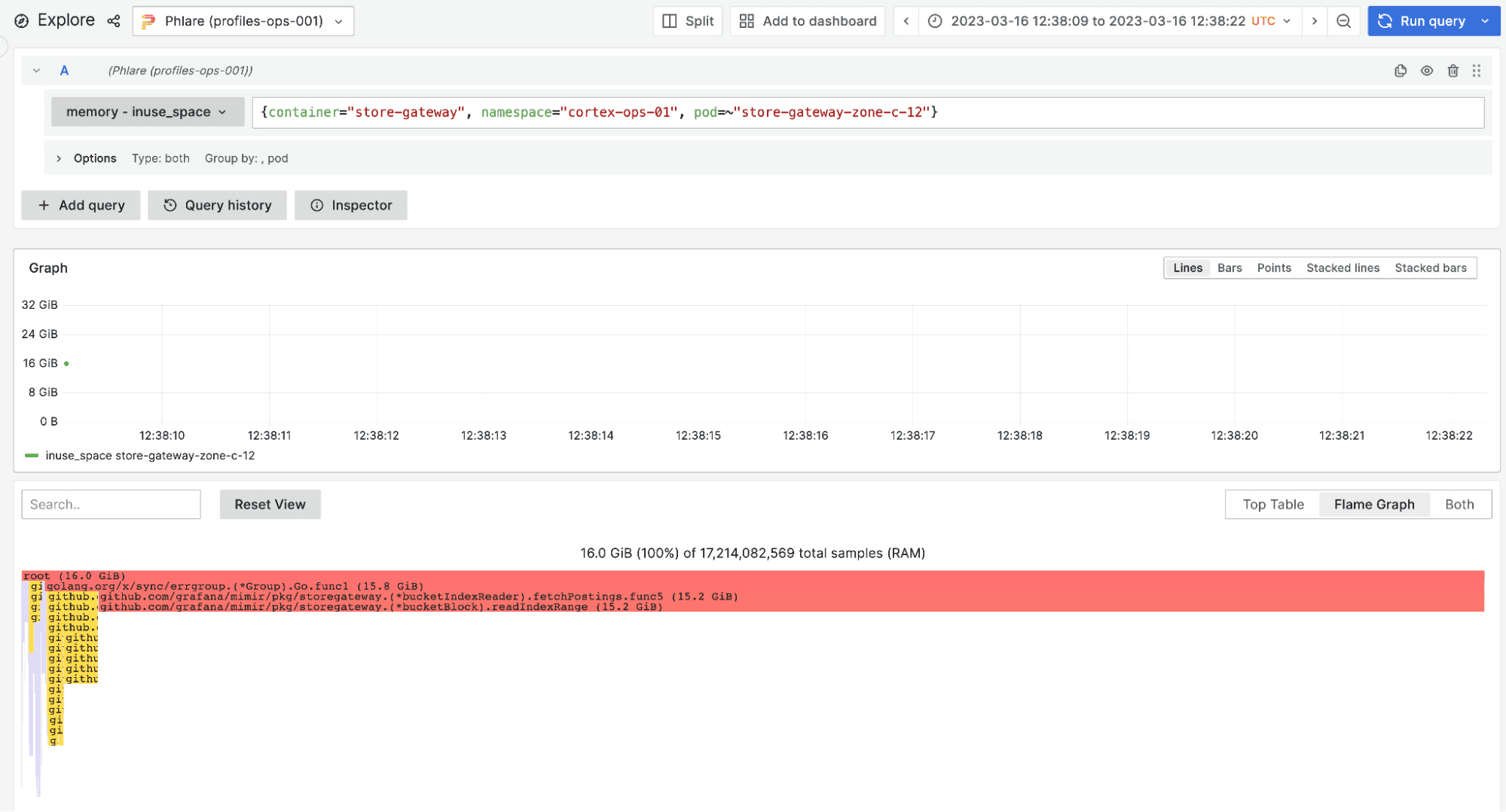
Series IDs are expected to be negligible compared to the size of the series labels and chunks of samples, but for some reason they weren’t. Below is a profile that shows that the function fetchPostings is taking up 15.2GiB out of the total 16GiB of heap in a store-gateway replica. It’s also important to note that the fetched series IDs are not only the IDs of the series effectively returned by the query. They also include IDs fetched during intermediate steps of the query execution, as we’ll see more in detail later on.
Active queries tracker in Mimir
Mimir has a feature that allows us to see which queries were being executed by a process when it crashed. This feature, called active queries tracker, is particularly useful to see exactly which queries were being executed at the time of the store-gateway OOM.
Mimir writes all incoming queries to a file and removes them from the file when they complete. If Mimir exits cleanly, there shouldn’t be any active queries in the file. If Mimir crashes, then the file contains all the queries that were being executed at the time of the crash. When Mimir starts up, it checks whether there were unfinished queries in the file and logs them to standard out, and we can query them in Loki.
When we looked at the active queries at the time of crashes a lot of them looked like this:
sum(avg_over_time(successful_requests_total:rate5m{service="cortex", slo="writes request error", cluster=~".+"}[5m15s]))
The above is a query from an SLO dashboard that engineers at Grafana Labs use. It calculates the average rate of successful requests over five minutes. At first glance, nothing in it stands out as particularly costly. In fact, the whole query selects only 38 series and returns a single series.
How simple Prometheus queries become the most expensive
Now let’s see what the store-gateway has to do to execute the above query. The responsibility of the store-gateway is to fetch all series that match successful_requests_total:rate5m{service="cortex", slo="writes request error", cluster=~".+"} and return them to the querier for the complete PromQL evaluation.
This is a high-level overview of how the store-gateway does this:
- Find all series IDs matching the
successful_requests_total:rate5mmetric name.- This is a single list of series IDs for all series of this metric.
- The metric is relatively low cardinality and this list contains only 1200 series IDs.
- Find all series IDs that match
service="cortex".- This matches roughly 6483 series.
- Find all series IDs that match
slo="writes request error”.- This is even a narrower set of series and matches only 798 series.
- Find all series IDs that match
cluster=~".+". This involves finding all the possible values ofclusterand creating a union of the series IDs from all the values.- Since these are all the possible values of the
clusterlabel and since almost all time series have that label, the union of these two sets is effectively almost as big as the list of all series IDs in the TSDB block. In our case, that was in the order of 80 million series.
- Intersect the series IDs from the four steps above to find the series IDs that match all four matchers in the query. (The metric name is also a matcher.)
- For this query, the final intersection selects 38 times series.
- For each series ID in the intersection, fetch the time series labels and chunks.
- On average each series has between 1KB and 2KB of chunks per 24-hour block, and its labels are usually below 1KB. This means that 38 series will generously take up less than 200KB of labels and chunks.
- This is usually the bulk of the work, but it’s omitted here for brevity.
- Return the labels and chunks to the querier.
It’s important to understand that the matchers aren’t used to filter out series one by one like a sequential scan in a SQL database. In Mimir (and Prometheus), series are looked up through an inverted index, where the matchers are only used to find the series matching each matcher individually and then the sets of matching series get intersected.
As you might have guessed, the culprit that was causing OOMs was bringing those 80 million series IDs in memory in step 4. Since each takes up 8 bytes of memory, 80 million IDs take up 640MB of memory. In comparison, the labels and chunks of the selected 38 series took less than 200KB of memory. Doing this for a single query is probably ok, but when one user query gets split and sharded into hundreds of partial queries, the effect of those 640MB can be amplified and easily lead to an out-of-memory error.
What makes this even more annoying is that, for the shown query, the cluster=~”.+” matcher does not actually filter out any of the series. In other words, even if the user ran that query without that matcher the result will be the same. We call these matchers “broad matchers.” This cluster matcher in particular comes with a 640MB cost and does not alter the outcome of the query.
In addition to that, queries sometimes come with multiple broad matchers (for example `namespace=~”.+”` and` pod=~”.+”`). They usually slip in from template variables in Grafana dashboards that are set to include all values. Sometimes these broad matchers filter out no series at all; sometimes they filter out a few series.
So how can we optimize Mimir when broad matchers are used in a query?
Optimizing queries with broad matchers
If we knew in advance that a matcher would be a broad matcher, we could avoid loading the list of series IDs that it matches. Then we could exclude the broad matcher from the inverted index lookup and only apply it to the set of series we get using the rest of the matchers. In this case, we would fetch more series, some of which might not match `cluster=~”.+”`, apply the matcher to filter them out, and then return the result. However, we cannot know in advance the selectivity of each matcher from each user query with precision, because we cannot predict what matchers a user will send.
While we can’t predict the selectivity of a matcher, we can make an educated guess about how many series the matcher will select. In other words, if matcher A selects a small number of series and matcher B selects a large number of series, we could only look up the inverted index to find the series matched by A and fetch them. Then apply matcher B on the fetched series one by one.
And this is what we did.
Using the layout of the inverted index in the Prometheus TSDB, we can infer the size in bytes of each series IDs list before we load it. Since the lists contain fixed-size entries, this immediately gives us how many series a list contains.
If we think of all matchers as the sets of series that they select, then we can put an upper bound on the number of series that the whole query selects. In our example above, we know that the query successful_requests_total:rate5m{service="cortex", slo="writes request error", cluster=~".+"} cannot select more than 798 series because that’s how many series the narrowest matcher selects - slo="writes request error”.
Using an estimated number of bytes that each series takes up, we find out that the query shouldn’t select more than 10MB of data. Another way to look at it is, if we were to only use the slo matcher and fetch all 798 series that it selects, then we wouldn’t fetch more than 10 MB of data. We can then apply the rest of the matchers on these 798 series to narrow them down to the 38 series that the user originally intended.
In practice, the optimization first analyzes the cardinality of each matcher and estimates their memory utilization. Then, it excludes all the matchers from the inverted index lookup that would result in a higher memory utilization, compared to the memory footprint of fetching some extra series that would be later removed by the excluded matchers. Finally, it fetches the series labels for the series found through the inverted index and filters out series not matching the matchers that were previously excluded.
Results
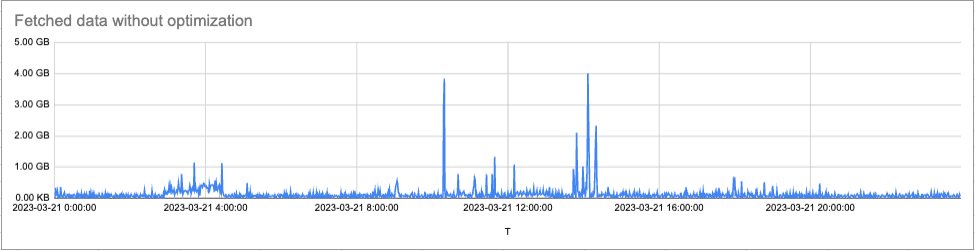
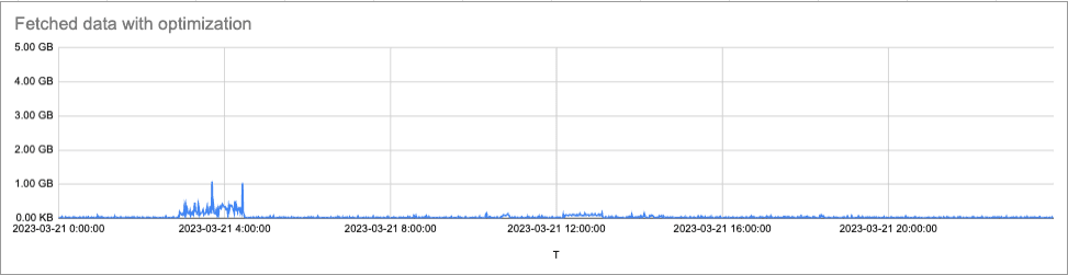
We implemented this approach and initially tested it offline, replaying all queries run in an internal Mimir cluster within a day. Below is the rate of fetched data per minute with and without the optimization. The initial test results were very promising. We saw a reduction of up to 69.6% of the total data that the store-gateway processes and a significant reduction in peaks.
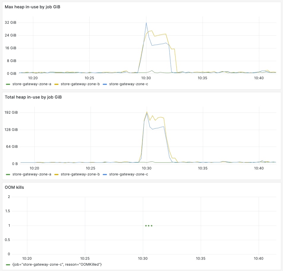
After more testing in dev and staging Mimir clusters, we rolled it out to production. We observed massive reduction in store-gateway memory utilization peaks and out-of-memory errors in production. Below is one example of a production cluster where we deployed the optimization only to store-gateway-zone-a. Store-gateways in zone b and c (no optimization enabled) spiked their go heap usage to 32GiB whereas zone a stayed just above 2GiB.
At Grafana Labs, we run all Mimir clusters on Kubernetes. To manage the compute resources of the store-gateway, we use resource limits and requests. The memory request is how much memory each store-gateway container has reserved. Because the memory that each store-gateway has requested is reserved exclusively for its own use, the memory request is a good proxy for the actual cost of compute memory that the store-gateway needs.
Reducing the memory spikes caused by lists of series IDs not only improved query performance and stability of the Mimir store-gateway. It also allowed us to reduce the memory requests for the store-gateway in some clusters by up to 64%, contributing to lower Mimir TCO. After rolling out this change across all Mimir clusters and measuring the effects, we found that we were able to reduce the store-gateway memory requests by 30%. In other words, the store-gateway can now handle the same load with, on average, 30% less memory.
More optimizations in Grafana Mimir
In our blog series about Grafana Mimir optimizations, we showed how we improved the query experience in Grafana Mimir with our work on the store-gateway, the component responsible for querying long-term storage.
In the first blog post, we introduced results streaming, which significantly alleviated the memory complexity of a query in the store-gateway. After this work, the store-gateway could serve much bigger queries and its memory was no longer a function of the size of response.
Next, we tackled how the store-gateway reads files from disk. We eliminated the unpredictable behavior of mmap in golang, which ultimately gave the store-gateway more consistent performance and reduced the interference between concurrent user queries.
Finally, as we described in this blog post, we optimized a specific set of queries that turned out to be more resource-intensive than we anticipated. We made use of the specific layout of the Prometheus TSDB block index to optimize how the store-gateway uses the inverted index and eliminated unnecessary lookups.
As we continue to refine the querying experience in Grafana Mimir, we have identified work to make the PromQL evaluation in the querier component complete in a streaming fashion. This is similar to the streaming work in the store-gateway, but will also improve how recently ingested samples are queried and decouple the memory footprint of queries from the size of their results. Stay tuned for more improvements in future Mimir releases!
Grafana Cloud is the easiest way to get started with metrics, logs, traces, and dashboards. We have a generous forever-free tier and plans for every use case. Sign up for free now!