Monitoring high cardinality jobs with Grafana, Grafana Loki, and Prometheus

Ricardo Liberato is a consultant building solutions for corporate clients using the power of the Grafana ecosystem to tackle problems beyond the data center and into the business realm. He can be reached at http://liberato.pt

Since 2006, I’ve been consulting for a Fortune 100 life sciences company building increasingly powerful observability solutions. We started with custom-built solutions, migrating to Grafana and Prometheus back in the Grafana 3 days. The company has a data lake of more than 3,000 nodes holding its data and load infrastructure, and we have been happily using Grafana to monitor it for six years now. 

In this post, I’d like to share my experience using Grafana, Prometheus, Grafana Loki, and our own custom-built exporters, and explain how we were able to leverage the deep synergies between Loki and Prometheus to monitor high cardinality jobs. 

But first, let me start with how we got here. 

When the Grafana Loki project was announced in 2018, we saw we could use it to go beyond infrastructure monitoring and start looking inside jobs to extract job-run performance information. That was something that had not been possible just with metrics due to two factors: Job runs are short-lived and cause an explosion in the number of series (high cardinality ruins Prometheus’s performance over time), and the information about what a job run has achieved was only available in logs.

By adding Grafana Loki to our existing Grafana and Prometheus monitoring, we were able to monitor the actual performance of jobs so we could know which tables were loaded and how often load cycles were completed for streaming loads. This enabled us to reduce cycle time for loads from 20 minutes to less than six minutes. By combining metrics with logs information, we were able to deeply understand where compute and memory were being efficiently used and where it was being wasted. This unlocked 40% savings on the cost of the cloud infrastructure supporting these stream jobs.

Now, I’ll go deeper into these two use cases and also highlight the job_exporter we built that leverages the symbiosis between Prometheus and Loki to break the high cardinality barrier.

Data-load technology setup

For background, our data lake is fed by more than 200 enterprise resource planning (ERP) systems and many custom databases. The data lake is updated by a combination of near real-time stream jobs and nightly batches, depending on the criticality of the data. Technologies involved in these loads include Informatica, Kafka, SpringXD, Databricks, Azure Data Factory, Spark, and Pivotal Gemfire.

We have three kinds of loads running across this infrastructure: 

1. Incremental loads, which are scheduled every four hours and carry reference data that doesn’t need to be updated in real time
2. Stream loads, which run continuously, loading operational information which has an SLA of hitting the data lakes 15 minutes from being produced in the ERPs
3. Machine learning jobs, also in Databricks, which add insight to the information in the data lakes

Use case no. 1: Job performance monitoring

Monitoring jobs is business-critical because it is the only way data from 100s or ERPs is made available both for analytics and modern applications built on top of the data lake. 

To effectively monitor jobs we need to know:

• What is running now and historically?
• How much resource are they taking up in the cloud infrastructure?
• How fresh is the information loaded?
• From which ERP is this information coming?
• Which tables are being loaded and with how many rows?

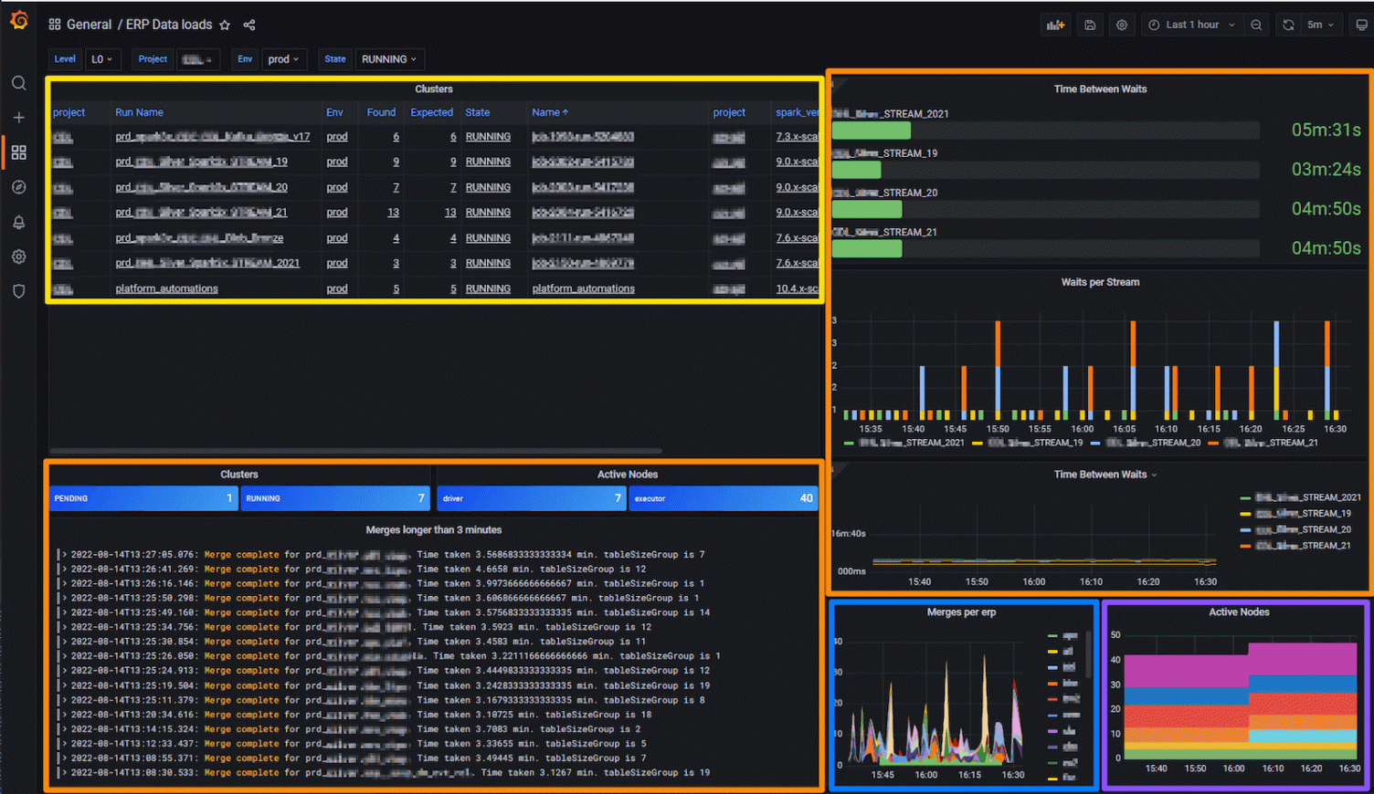
We’ve configured our main Grafana dashboard so we have access to all of this information across dozens of jobs in one screen.

Below, the panel highlighted in yellow shows cluster and job status; the orange one contains job performance data; the blue has ERP distribution; and the one outlined in purple is where we can see how many nodes are active in this environment over time.

Here’s a closer look at what we are observing: 

Cluster performance

In the Clusters Panel (outlined in yellow), we can see information comparing the responses from the Job Controller (Databricks API) and information gathered from the jobs by the Grafana Agent. We compare the Expected and Found columns to alert if the cluster isn’t healthy. The bottom right panel shows the same information in a stacked chart, which has a direct correlation to how much we are spending on compute at any moment in time.

Job performance

In the section highlighted in orange, we monitor the performance of the load jobs themselves — specifically merges longer than three minutes. You can see raw log lines, which are aggregated into Prometheus using Loki recording rules but are also still available to view from Loki.

We find Grafana’s unique ability to have both the raw data and the aggregates correlated across metrics and logs extremely powerful, and we have used it in multiple parts of our solution.

Dozens of megabytes of logs are written per minute by the processing nodes, and among them are lines that tell us when a stream job completes a cycle. We have a strong SLA per stream of 15 minutes per cycle, and in this dashboard we can view current and historic performance as well as generate alerts.

We use Loki’s recording rules to capture this information in Prometheus for both quick display and trend analysis. We found those rules to be extremely useful, enabling time series calculations on log information that just wouldn’t be possible (or at the very least extremely slow) with just a logging solution.

To monitor tables and ERP distribution, we built separate drill-down dashboards that aggregate information while allowing us to filter to see only one project or even a specific table. Here’s an example:

With these two dashboards, we are able to not only control operations, but we also feed back insights to development teams so they tune the loads based on actual production performance. We’ve been able to cut cycle time by more than threefold in six months, increasing the freshness of data used for decision making. At the same time, we’re able to alert on any slow-downs or connection problems with any of the data sources.

Use case no. 2: Cost-reduction for cloud jobs

When you’re running hundreds of nodes, cloud compute resources can add up quickly. To avoid ballooning costs, you want to identify opportunities that can help you do one of two things: tune the load to better take advantage of the resources allocated to it, or reduce unneeded resource allocation.

Below you can see the heartbeat of a stream job, which displays CPU and memory information from Prometheus along with merge timestamps collected from Loki, all in one graph. In this panel, we also monitor overall CPU usage over time.

With the insights the rich Grafana visualization provides, we were able to help the development teams focus their optimization efforts, achieving SLA while reducing costs by 40%.

We were also able to see that static cluster allocation causes resource wastage, and we’ve trained a machine-learning model to predict needed resources and then scale up or down the clusters we use. This is now in pilot and is already forecast to provide another 30% in savings.

Solution outline

Our job monitoring journey started by implementing one-off solutions for Databricks and for Azure Data Factory. The learnings from these two implementations — and the need to extend to more platforms — led us to build a generic job_exporter that is easily extensible and supports:

• Databricks
• Native Spark
• Azure Data Factory
• SpringXD
• Informatica PowerCenter

The abstraction is based on the following data flow, replacing Job Control Engine with any of the above.

We have four flows of information which are seamlessly integrated with Prometheus and Loki by using labels in Grafana.

In Prometheus, we store two flows:

• Current job execution status information stored in Prometheus metrics (avoiding high cardinality items like job id or table)
• Metrics collected by the Grafana Agent and jmx exporter

In Loki, we split information into two main log streams:

• Status log stream (this has the high cardinality metrics as well as all information collected on the job execution as a json payload)
• Job execution streams (tagging key execution lines using Promtail built into the Grafana Agent)

All four flows are seamlessly integrated through labels that identify which job execution they came from.

Job exporter internals

The job exporter is a highly tuned golang binary, which we can configure at run time through a yaml file to support any of the systems above. It can be easily extended to support more job control engines.

The job_exporter reads current state for jobs from APIs or databases and writes the low cardinality data to Prometheus. At the same time, it is also detecting state changes which it writes to logs in Loki with the same labels. Together with the state changes, we write the full payload of information to logs that are collected by Loki. This would cause a cardinality explosion if written to Prometheus, yet it remains easily accessible in Loki.

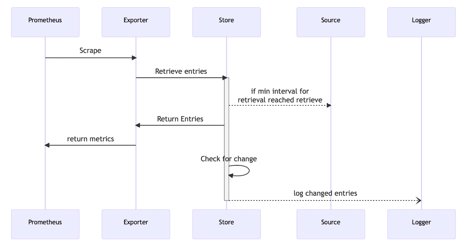
The exporter consists of the following dynamic configured actors that are configurable at start time in a yaml file:

• Exporter: a Prometheus exporter implementing a probe and metrics endpoint
• Store: an in-memory cache that allows us to avoid calling a source when we would exceed API quotas
• Logger: this writes a json log of mutations, including the whole payload discovered
• Source: named sources that implement the data collection specific to each job engine and map it to the generic framework

The following diagram shows the interaction between the different actors:

Conclusion

Implementing the two use cases I’ve described showed us that Grafana Loki and Prometheus are much more powerful when treated not as separate components but as a mutually reinforcing pair. Using them together allowed us to build solutions that far surpass what can be built with either of them.

I hope this inspires you to look for what you can achieve by breaking the high cardinality barrier.

Want to share your Grafana story and dashboards with the community? Drop us a note at stories@grafana.com.