How summary metrics work in Prometheus

A summary is a metric type in Prometheus that can be used to monitor latencies (or other distributions like request sizes). For example, when you monitor a REST endpoint you can use a summary and configure it to provide the 95th percentile of the latency. If that percentile is 120ms that means that 95% of the calls were faster than 120ms, and 5% were slower.

Summary metrics are implemented in the Prometheus client libraries, like client_golang or client_java. You call the library in your REST application, and the library will calculate the percentiles for you.

Understanding the underlying algorithm used in these libraries is hard. You will see code comments referring to a research paper named “Effective computation of biased quantiles over data streams” by Graham Cormode, Flip Korn, S. Muthukrishnan, and Divesh Srivastava, often referred to as CKMS by the initials of the authors’ last names. If you are like me, you will find that paper hard to read.

This blog post is an attempt to summarize the CKMS algorithm in simple terms.

Do I really need to know this?

No. You can use summary metrics without knowing how they work internally. There are other things that you should know when measuring latencies, like when to use summaries and when to use histograms, but the algorithm used for calculating percentiles is none of them.

However, it is pretty interesting to have a look under the hood, and understanding how the CKMS algorithm works will help you avoid some common pitfalls when monitoring latencies or other distributions.

Terminology

The terms percentile and quantile mean basically the same thing:

• A percentile is represented as a percentage between 0 and 100. For example, “the 95th percentile of a latency distribution is 120ms” means that 95% of observations in that distribution are faster than 120ms and 5% are slower than 120ms.
• A φ-quantile (0 ≤ φ ≤ 1) is represented as a value between 0 and 1. For example, the 0.95 φ-quantile of a latency distribution is the same as the 95th percentile of that latency distribution.

In this blog post, we use quantile as a short name for φ-quantile, following the terminology used in the CKMS paper.

Exact quantiles

Calculating an exact quantile is trivial, but it costs a lot of memory because you need to store all latency observations in a sorted list. Let’s introduce some variables:

• n: The total number of observations (i.e., the size of the sorted list).
• rank: The position of an observation in the sorted list.

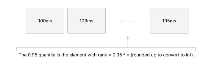
Given a complete sorted list of observations, it is easy to find the quantile. For example, if you are looking for the 0.95 quantile, you just need to take the element with *rank = 0.95*n *(i.e., the element at position 0.95*n rounded up to convert to int).

Data model for a compressed list

Storing a complete list of observed latencies obviously takes too much memory for real-world applications. Therefore, the CKMS algorithm defines a compress function that discards observations from the list, keeping only a small number of samples.

The downside is that we can no longer know the exact rank of the samples: When we insert a new observation into the list of samples, it is impossible to say exactly at which position it would have ended up in the complete list.

However, we can keep track of the minimum and maximum possible rank for each sample:

Note that the intervals of the possible ranks overlap. However, the minimum possible rank of each sample is always at least 1 larger than the minimum possible rank of its predecessor.

In practice, it is inconvenient to store the absolute minimum and maximum possible rank for each sample, because when we insert a new sample, the ranks of all samples to the right need to be incremented by 1.

Therefore, the CKMS algorithm stores deltas instead of absolute values:

• g: The difference between the minimum rank of this sample and the minimum rank of its predecessor.
• delta: The size of the interval, i.e. maximum possible rank minus minimum possible rank.

With that encoding, the list of samples above looks like this:

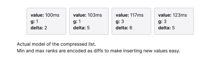
Using that representation, we can insert new samples without updating the existing ones in the list.

We can easily calculate the minimum possible rank of a sample by adding its g value to the sum of g values of all predecessors in the list. The maximum possible rank is the minimum plus delta.

Limiting the error: an upper bound for delta

The API of summary metrics in Prometheus client libraries allows users to define an allowed error margin. For example, in client_java the API looks like this:

java Copy

Summary.build("name", "help message")
	.quantile(0.95, 0.01)
	.register();

In the example, the allowable error of 0.01 means that we are targeting the 0.95 quantile, but we are happy with any value between the 0.94 quantile and the 0.96 quantile.

In order to guarantee that the result is within these bounds, we need to set an upper bound for delta, i.e., we need to restrict the size of the range of possible rank values for each sample.

A trivial upper bound for delta could be derived as follows: If we want to stay between the 0.94 and the 0.96 quantile, the minimum allowable rank is 0.94 times the total number of observations, and the maximum allowable rank is 0.96 times the total number of observations. Subtract max - min, and you get an upper bound for delta.

However, the CKMS algorithm is more clever than that: We need that strict bound only around the 0.95 quantile. We are not interested in other quantiles, so we can relax constraints around other quantiles.

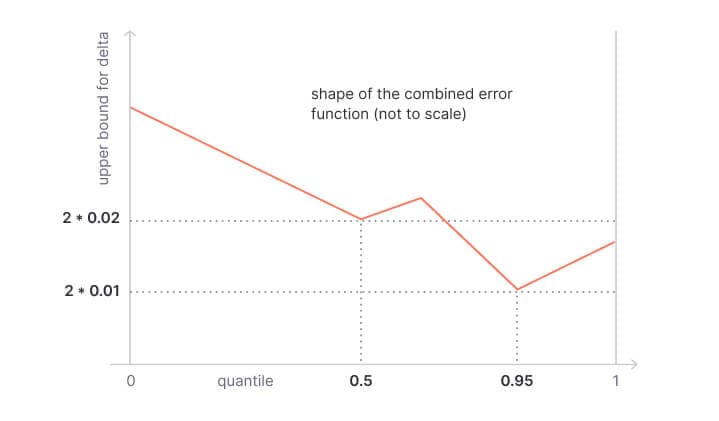
The CKMS algorithm defines an error function that keeps a strict upper bound on the target quantile, but relaxes the error margin the more you go to the left or the right.

The figure above shows the error function with 0.95 as the target quantile and 0.01 allowable error. That means, the actual result will be between the 0.94 quantile and the 0.96 quantile.

Here’s another example: It shows the error function with 0.5 as the target quantile (the median) and 0.02 as allowable error. That means, the actual result will be between the 0.48 quantile and the 0.52 quantile.

Interestingly, you can keep track of multiple quantiles by combining these functions.

java Copy

Summary.build("name", "help message")
	.quantile(0.95, 0.01)
	.quantile(0.5, 0.02)
	.register();

The combined error function guarantees a 0.5 quantile with allowable error 0.02 and a 0.95 quantile with allowable error 0.01.

The algorithm

The algorithm itself is straightforward: It defines the functions insert and compress, and makes sure that both functions guarantee that delta is never greater than allowed by the error function.

Insert

The list of samples is sorted by the observed values. When inserting a new value, we first need to find its position in the sorted list, and then we add a new entry with the following values:

• g=1: The minimum rank is at least 1 more than the minimum rank of the predecessor.
• delta = maximum allowed error of the predecessor - 1: The uncertainty in rank of the new entry is at least 1 less than the maximum allowed uncertainty of the predecessor before the new element was inserted.

When we insert a sample at the beginning of the list, or at the end of the list, or to an empty list, we set g=1 and delta=0.

Compress

Every once in a while compress is called to remove entries from the list. As an example, client_java calls compress periodically for each 128 insertions.

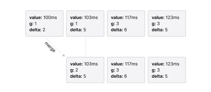
The compress function scans the list and merges adjacent nodes when this does not violate the error function. The merged node is initialized as follows:

• value: The value of the right node, discarding the value of the left node.
• g: The sum of the g’s of the left and right node. As we took the value of the right node, the difference between the minimum rank of the merged node and its predecessor is the sum of the minimum distances of the merged nodes.
• delta: The delta of the right node.

Here’s an example of merging the first two nodes:

Evaluation

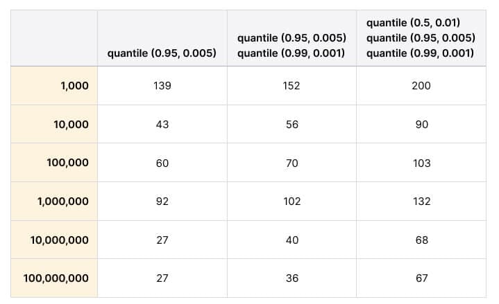
The compression rate is mind-blowing. I inserted between 1,000 and 100,000,000 random values and repeated this with tracking one, two, and three quantiles. The number of samples in the compressed list at the end of each run remained well below 100 in most runs, and it did not increase with the increased input size.

I used the client_java implementation for the evaluation, the source code for the evaluation is here.

Pitfalls

There are some pitfalls with the CKMS approach:

• You cannot aggregate across multiple instances. For example, if you have one summary representing latencies observed on server A, and another summary representing latencies observed on server B, then there is no way to combine these separately computed summaries.
• The error margin is relative to the rank, not relative to the observed value. For long-tail latency distributions this might make a huge difference. For example, the 0.94 quantile might be 120ms, but the 0.96 quantile might be far out at 2343ms. By accepting any value between the 0.94 and 0.96 quantile you will be accepting any value between 120ms and 2343ms.

Both can be addressed by using histograms instead of summaries, and by calculating quantiles from these histograms using the histogram_quantile() function of the Prometheus query language. However, you can use summaries without any prior knowledge about the distribution you want to monitor, while current Prometheus histograms require a priori definition of bucket boundaries.

Notes and implementation details

The goal of this blog post is to give you a high-level overview of how the implementation of summary metrics in Prometheus client libraries works internally. There are some details that I left out to make the post easier to read:

• The upper bound for delta used in the paper is actually not on delta, but on g+delta. This makes the calculation overly conservative, but the overtight bound helps to make accuracy guarantees.
• Inserts are implemented in batches. For example, client_java collects 128 values in a buffer and flushes the values to the compressed list when the buffer is full (or when the Prometheus server scrapes).
• You don’t want to get latency metrics for the entire runtime of an application. You want to look at a reasonable time interval. For example, client_java implements a configurable sliding window which is 10 minutes by default.

Related work

The CKMS algorithm was published in 2005 and is relatively old (which doesn’t mean it’s not fit for purpose). Newer research on quantiles includes:

• Space- and Time-Efficient Deterministic Algorithms for Biased Quantiles over Data Streams, a newer paper by the same authors as CKMS.
• Computing Extremely Accurate Quantiles Using t-Digests, which comes with a reference implementation in Java and independent implementations in Go and Python. Allows separately computed summaries to be combined with no loss in accuracy.