
How sparse histograms can improve efficiency, precision, and mergeability in Prometheus TSDB
Grafana Labs recently hosted its first company-wide hackathon, and we joined forces with Björn “Beorn” Rabenstein to bring sparse high-resolution histograms in Prometheus TSDB into a working prototype.
The Prometheus TSDB has gained experimental support to store and retrieve these new sparse high-resolution histograms. At PromCon 2021, we presented our exciting, fresh-off-the-presses results from the ongoing project. (For a deeper dive into sparse histograms, check out the in-depth design doc that Björn wrote.)

You can also check out the latest information about sparse histograms that was presented during Grafana Labs’ ObservabilityCON 2021.
What we know about histograms in Prometheus
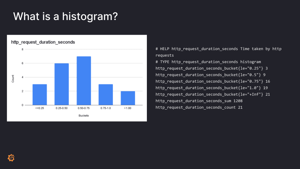
What is a histogram anyway?
In short, a histogram is a way to categorize your numeric observations into ranges and count the number of observations for each range, which is useful for looking at the distribution of data such as, for example, latency metrics.
The current implementation in Prometheus is shown below. It uses a series for each bucket. Each series has a label declaring the upper bound and the number of observations with a value less or equal to that bound. In other words, the counts are stored cumulatively (each bucket includes the count of smaller buckets). Then there are also some additional series, such as _sum series with the sum of all the observations, and the _count which is the count of all observations.
There are a few problems, however, with the current implementation of histograms.
First, users have to manually define their buckets. That means it’s basically guesswork around what the values should be, which leaves users hoping data won’t go out of bounds or lose precision. It’s a clunky method, and we would rather establish the right bucket sizes automatically.
Another issue is that queries require aggregation both across time and across labels, which doesn’t work when you have histograms with different bucket layouts. Ideally, different layouts should be chosen so that they are compatible, and they could be merged together to avoid losing precision.
There should also be accurate estimations. There needs to be a low error rate so that you can compute correct quantile estimations. This requires smaller buckets, and more buckets for unforeseen observations.
Finally, we believe that if we can lower the costs of histograms, then we can make partitioning much more feasible. We suspect that many histogram users don’t partition as much as they can, such as partitioning by an HTTP status code label or by a route or a path label. But if we make histograms much cheaper, then you can partition as much as you want.
Inside the prototype
Here’s an example demonstrating the type of insights you can get with high-resolution sparse histograms by using a heatmap. Although, of course, there are many more use cases and visualizations for the new histograms.
The width of the “band” shows how uniform the observations were. From left to right, we first see the latency creep up across the board and then stabilize. We also see more requests (red and orange buckets). After some time, a new canary was deployed and results in a fraction of requests being faster. Once the rollout was complete, latencies became more consistent (and lower, overall) but less predictable because the observations were spread out over a large range.
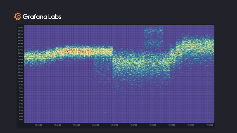
After some time, part of the system started behaving strangely, and the latency shot up. There are two bands of slowness which could be the result of a heavy operation or some cold caches. The heat map shows the exact time when the issue started and when the issue stopped. Once the issue stopped, the latency continued increasing and then stabilized.
This is one example of the visualization and insights that we would like to get from high-resolution histograms, but it’s not feasible right now because of the expensive buckets in Prometheus.
Let’s discuss the exposition and TSDB encoding we’ve implemented in our prototype, as well as the benchmarks we’ve run.
Exposition code

The instrumentation for sparse histograms is based on the current instrumentation. In the code above, the orange line exposes the conventional histograms. The sparse buckets factor defines the precision of your sparse histogram and how much growth there is as you go from one bucket to the next. We dynamically allocate as many buckets as needed to accommodate the data.
In theory, it can just grow infinitely without setting a limit. But to restrict resource usage, you can set a limit. In this case, we set a maximum number of 150 buckets.
To honor the limit, the exposition will automatically start a fresh chunk with only the buckets that are currently in use (this is akin to counter reset). There’s a limit to how often this can happen, and here we limit it to once per hour. We expect this to be typically enough to stay within the limit. If not, the precision is automatically decreased (buckets widened) to reduce the number of buckets.
Chunk encoding (simplified)

After the data gets scraped, how does it actually get saved into histogram chunks? There are two main components: At the beginning of the chunk, you have your metadata that describes the exact shape of your histogram. Then there are the individual histogram samples.
For the metadata there are two key entries: First, there is the schema, which is simply a number that describes the growth factor. In the previous example, we showed a growth factor of 1.1. This value gets encoded as a simple integer.
Then we declare which buckets are actually being used. In theory, you could have an infinite number of buckets. Some of these buckets might be used for data. Some buckets might need to be skipped because they don’t have any data. So we simply encode this in a list of entries that declare a certain number of skipped (unused) buckets followed by a number of used buckets (for which we will encode data).
This is why we call them sparse histograms. They are an efficient way to avoid the overhead of maintaining all the buckets that are not used.
Note that just these two metadata items alone describe the complete, exact shape of the histogram.
As far as the actual data, we’re inspired by the current XOR encoding of normal time series in Prometheus, except in this case there are more fields and a variable number of fields for the buckets (the amount can be deduced from the metadata).
In the first histogram sample that comes in, we’re storing all the fields raw as integers, as floats, and as a sequence of integers. The second histogram will store deltas. For the rest of the histograms from the third histogram onwards, we store delta of delta everywhere. The one exception is the sum field. Because it’s a floating point number, we use the XOR encoding just like the standard XOR encoding of time series.
All of this data gets written into a bitstream, which then gets serialized as a chunk of bytes. A chunk holds the complete metadata describing the histogram format as well as all the histogram samples.
The sparse histograms testing setup
We instrumented the Cortex gateway on our Grafana Cloud dev clusters with both conventional and sparse high-resolution histograms. The Cortex gateway is the component which sits in front of our Cortex clusters and all the read and write traffic goes through it. We also set up two Prometheus instances — one of them only scraping the conventional histograms and the other only scraping the high-resolution sparse histograms. Then we compared the storage at saturation, which means all the buckets that had to be filled were full and there was less sparseness.
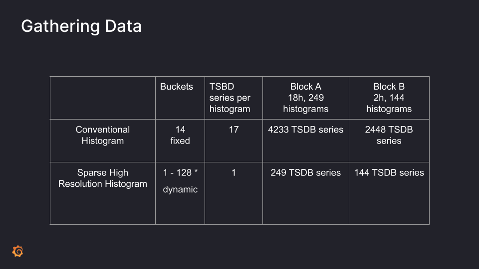
The table above shows what the data looked like in both the scenarios.
In the conventional histograms we have 14 series — one for each defined bucket — as well as the infinite bucket, the sum and count series, resulting in 17 TSDB series per histogram.
For sparse high-resolution histograms, the number of buckets varies in our data for different histogram series. We saw that it varied between one bucket to 128 buckets, and it’s dynamic. Because all of these buckets are stored in the same chunk, we only need one time series in the TSDB to represent a histogram and all its buckets.
So we have two data blocks under observation — Block A scraped data for 18 hours and had 249 histograms. Similarly Block B scraped data for two hours and had 144 histograms. For the number of series, it’s a multiple of 17 for the conventional and a multiple of one for the sparse. Both of them scrape the same thing, yet Block A has nearly double the number of histograms because there was a rollout of Cortex gateway in between which resulted in more histograms because of label change. With sparse histograms, we can use many more buckets, using a fraction of the series, and thus index cost. We will measure the precise index savings in our benchmark results below.
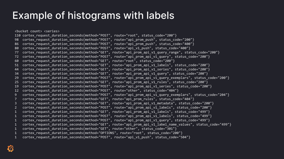
Above is a snapshot of dynamic buckets of few of the series from the blocks of the sparse histogram. You can see that the number of buckets vary in huge numbers.
For example, a PromQL query can be arbitrarily cheap or expensive and thus result in a variety of different latencies; hence, we need more buckets. But other types of responses, such as errors or a gateway timeout, will typically come back with a consistent latency. Any such histograms only need very few buckets, possibly just one. These result in lightweight series.
This ultimately shows that partitioning histograms into multiple histograms with different labels may be too expensive because the number of buckets is dynamic.
TSDB benchmarks
Now let’s look at our benchmark results.

In the first column, there’s a reduction in index size of about 93% for the block. And if you look carefully, it is a 17x reduction, which reflects the ratio between the number of series required for conventional vs. sparse histogram.
If you look at the chunks, though we have more buckets in this histogram, you will still get efficient encoding. There’s roughly 43% and 48% reduction in its size. And when you combine both the sizes of the index and chunks, the overall reduction is about 40 to 60%. This also means the memory that Prometheus would take will be similarly less for histograms because the in-memory Head block is using the same chunk encoding as used in the block. Plus, series labels take a lot of memory usually, and that’s going to reduce with a single series per histogram. So there comes the overall savings in memory and in space.
What’s next for sparse histograms?
To recap, our prototype of sparse histograms in Prometheus removes the hassle of defining buckets and enables easy aggregation and merging of histograms.
In our tests, we saw a precision increase (due to the finer buckets) from 43% to 4.3%, a significant reduction of storage, and a 93% index reduction. The index largely dictates operational cost and resource usage so these results look promising.
You can put the index savings to good use because the new sparse histograms also make partitioning feasible. As observed, partitioning scales sublinearly, as only those series that need many buckets will use them, and many will be more lightweight. In contrast, current conventional histograms will allocate all buckets/series for all partitioned histograms.
The work that we have done up until now only contains scraping and ingesting into the TSDB and retrieving raw histograms at the TSDB layer. But we have a lot more work to be done!
The main work on our radar is the PromQL support, so that PromQL can natively work with these sparse histograms. We would also like to create sparse histograms in recording rules using PromQL. There also needs to be a compatibility layer to bridge the conventional and sparse histograms so that they can work together. Checkout the exploratory doc for the PromQL work for more details that Björn published after our PromCon talk.
We also want to play with more data, determine the query cost, and because there is a big reduction in index, we think that there ultimately will be a reduction in lookup cost for these histograms.
If you’re interested in the code, you can check the sparsehistogram branches of the Prometheus project and the client_golang repositories. We would love to hear what you think!
You can find the slides from our PromCon NA 2021 talk here.

